Kinematic driver: cloud and precipitation with P3

This example uses PrescribedDynamics to lift moist air through a vertical column at 2 m/s. P3Microphysics predicts cloud droplets, rain, ice, and liquid water carried on ice, with a prognostic vapor excess over liquid and aerosol activation. Velocity is prescribed while transport, thermodynamics, and microphysics evolve. We use liquid–ice potential temperature, the default thermodynamic formulation, explicitly selected below for clarity.

This is an open column: moist air enters at the bottom, air leaves at the top, and hydrometeors can sediment out. The rising-parcel example instead retains all water in a closed moving parcel. This setup demonstrates the ingredients of a kinematic microphysics comparison; it is not a reproduction of the upstream P3 kin1d benchmark.

using Oceananigansusing Oceananigans.Unitsusing Breezeusing Breeze.Microphysics.PredictedParticleProperties: AerosolActivation, AerosolModeusing CairoMakieusing Printf

Grid and background atmosphere

The column extends through the troposphere into the lower stratosphere. We construct hydrostatic pressure and density using the same potential temperature profile used to initialize the model. The atmosphere starts at 80% relative humidity over liquid water, with no condensate.

Nz = 100Lz = 20kilometersgrid = RectilinearGrid(CPU(); size=Nz, z=(0, Lz), topology=(Flat, Flat, Bounded))constants = ThermodynamicConstants()θ₀ = 300p₀ = 1e5ℋ₀ = 0.8zᵗʳ = 12kilometersθᵗʳ = 343Tᵗʳ = 213g = constants.gravitational_accelerationcᵖᵈ = constants.dry_air.heat_capacityfunction θ_initial(z)    θ_troposphere = θ₀ + (θᵗʳ - θ₀) * (z / zᵗʳ)^(5/4)    θ_stratosphere = θᵗʳ * exp(g / (cᵖᵈ * Tᵗʳ) * (z - zᵗʳ))    return ifelse(z ≤ zᵗʳ, θ_troposphere, θ_stratosphere)endreference_state = ReferenceState(grid, constants;                                 base_pressure = p₀,                                 potential_temperature = θ_initial)

ReferenceState{Float64}(p₀=100000.0, θ₀=300.0, pˢᵗ=100000.0)

Prescribed ascent and P3

Uniform vertical velocity does not satisfy ∂z(ρw) = 0 for a stratified density profile. divergence_correction=true compensates for that mass-flux divergence in the transported specific quantities. The flow remains prescribed even as latent heating changes the temperature.

P3's vapor_excess=PrognosticVaporExcess() adds ρδqᵛ⁺ˡ, the density-weighted vapor excess over liquid. Aerosol activation also predicts cloud droplet number and the remaining aerosol reservoir. Number mixing ratios are in kg⁻¹.

W₀ = 2nᵃ₀ = 3e8dynamics = PrescribedDynamics(reference_state; divergence_correction=true)aerosol = AerosolActivation(AerosolMode(number_mixing_ratio=nᵃ₀); prognostic=true)microphysics = P3Microphysics(; aerosol, vapor_excess=PrognosticVaporExcess())

PredictedParticlePropertiesMicrophysics
├── ρʷ: 1000.0 kg/m³
├── qmin: 1.0e-14 kg/kg
├── ice: IceParticles
├── rain: RainDrops
├── cloud: CloudDroplets
├── process_rates: ProcessRate
├── negative_moisture_correction: SpeciesBorrowing(vertical_borrowing = nothing)
├── aerosol: AerosolActivation(1 mode, prognostic reservoir)
└── warm_rain_scheme: KhairoutdinovKogan2000

Incoming air and precipitation boundaries

At the surface, pressure equals the standard potential-temperature reference pressure, so the condensate-free inflow has T = θ₀. Its moisture and vapor excess are calculated from the same relative humidity. Fresh aerosol enters with the air; all incoming hydrometeor mass and number are zero. P3's default open precipitation boundary allows sedimentation out of the column.

ρ₀ = surface_density(reference_state)qᵛ⁺ˡ₀ = saturation_specific_humidity(θ₀, ρ₀, constants, PlanarLiquidSurface())qᵗ₀ = ℋ₀ * qᵛ⁺ˡ₀δqᵛ⁺ˡ₀ = qᵗ₀ - qᵛ⁺ˡ₀microphysical_bcs = NamedTuple(name => FieldBoundaryConditions(bottom=ValueBoundaryCondition(0))                              for name in prognostic_field_names(microphysics))boundary_conditions = merge(microphysical_bcs,    (; ρθ = FieldBoundaryConditions(bottom=ValueBoundaryCondition(ρ₀ * θ₀)),       ρqᵗ = FieldBoundaryConditions(bottom=ValueBoundaryCondition(ρ₀ * qᵗ₀)),       ρδqᵛ⁺ˡ = FieldBoundaryConditions(bottom=ValueBoundaryCondition(ρ₀ * δqᵛ⁺ˡ₀)),       ρnᵃ = FieldBoundaryConditions(bottom=ValueBoundaryCondition(ρ₀ * nᵃ₀)),       w = FieldBoundaryConditions(bottom=NormalFlowBoundaryCondition(W₀),                                   top=NormalFlowBoundaryCondition(W₀))))model = AtmosphereModel(grid; dynamics, microphysics, boundary_conditions,                        formulation = :LiquidIcePotentialTemperature,                        advection = WENO(order=5),                        thermodynamic_constants = constants)

AtmosphereModel{CPU, RectilinearGrid}(time = 0 seconds, iteration = 0)
├── grid: 1×1×100 RectilinearGrid{Float64, Flat, Flat, Bounded} on CPU with 0×0×3 halo
├── dynamics: PrescribedDynamics
├── formulation: LiquidIcePotentialTemperatureFormulation
├── thermodynamic_constants: ThermodynamicConstants{Float64}
├── timestepper: SSPRungeKutta3
├── advection scheme: 
│   ├── momentum: WENO{3, Float64, Oceananigans.Utils.BackendOptimizedDivision}(order=5)
│   ├── ρθ: WENO{3, Float64, Oceananigans.Utils.BackendOptimizedDivision}(order=5)
│   ├── ρqᵛ: WENO{3, Float64, Oceananigans.Utils.BackendOptimizedDivision}(order=5)
│   ├── ρqᶜˡ: WENO{3, Float64, Oceananigans.Utils.BackendOptimizedDivision}(order=5)
│   ├── ρnᶜˡ: WENO{3, Float64, Oceananigans.Utils.BackendOptimizedDivision}(order=5)
│   ├── ρqʳ: WENO{3, Float64, Oceananigans.Utils.BackendOptimizedDivision}(order=5)
│   ├── ρnʳ: WENO{3, Float64, Oceananigans.Utils.BackendOptimizedDivision}(order=5)
│   ├── ρqⁱ: WENO{3, Float64, Oceananigans.Utils.BackendOptimizedDivision}(order=5)
│   ├── ρnⁱ: WENO{3, Float64, Oceananigans.Utils.BackendOptimizedDivision}(order=5)
│   ├── ρqᶠ: WENO{3, Float64, Oceananigans.Utils.BackendOptimizedDivision}(order=5)
│   ├── ρbᶠ: WENO{3, Float64, Oceananigans.Utils.BackendOptimizedDivision}(order=5)
│   ├── ρqʷⁱ: WENO{3, Float64, Oceananigans.Utils.BackendOptimizedDivision}(order=5)
│   ├── ρδqᵛ⁺ˡ: WENO{3, Float64, Oceananigans.Utils.BackendOptimizedDivision}(order=5)
│   └── ρnᵃ: WENO{3, Float64, Oceananigans.Utils.BackendOptimizedDivision}(order=5)
├── forcing: @NamedTuple{ρθ::Returns{Float64}, ρqᵛ::Returns{Float64}, ρqᶜˡ::Returns{Float64}, ρnᶜˡ::Returns{Float64}, ρqʳ::Returns{Float64}, ρnʳ::Returns{Float64}, ρqⁱ::Returns{Float64}, ρnⁱ::Returns{Float64}, ρqᶠ::Returns{Float64}, ρbᶠ::Returns{Float64}, ρqʷⁱ::Returns{Float64}, ρδqᵛ⁺ˡ::Returns{Float64}, ρnᵃ::Returns{Float64}, ρE::Returns{Float64}}
├── tracers: ()
├── coriolis: Nothing
└── microphysics: PredictedParticlePropertiesMicrophysics

Initializing the vapor excess

First initialize the thermodynamic state. Then initialize the density-weighted vapor excess from that state, so the prognostic starts with the actual vapor deficit. This second set! depends on the temperature and moisture established by the first.

set!(model; θ=θ_initial, ℋ=ℋ₀, w=W₀)μ = model.microphysical_fieldsρ = reference_state.densityqᵛ⁺ˡ = SaturationSpecificHumidity(model)set!(model; ρδqᵛ⁺ˡ=ρ * (μ.qᵛ - qᵛ⁺ˡ))

Simulation and output

Run for 3600 s, saving profiles every 30 s. The output retains both the prognostic and diagnosed vapor excess, along with mass and number concentrations, for subsequent comparisons. The vapor excess δqᵛ⁺ˡ has units of kg/kg; it is not the dimensionless supersaturation 𝒮.

simulation = Simulation(model; Δt=1, stop_time=60minutes)Oceananigans.Diagnostics.erroring_NaNChecker!(simulation)diagnosed_δqᵛ⁺ˡ = Field(μ.qᵛ - qᵛ⁺ˡ)outputs = (; T = model.temperature,             μ.qᵛ, μ.qᶜˡ, μ.qʳ, μ.qⁱ, μ.qʷⁱ,             μ.nᶜˡ, μ.nʳ, μ.nⁱ, μ.nᵃ, μ.δqᵛ⁺ˡ, diagnosed_δqᵛ⁺ˡ)filename = "kinematic_driver_p3.jld2"simulation.output_writers[:profiles] = JLD2Writer(model, outputs;                                                 filename,                                                 schedule = TimeInterval(30),                                                 overwrite_files = true)function progress(sim)    μ = sim.model.microphysical_fields    @info @sprintf("t = %s, max cloud = %.2e, rain = %.2e, ice = %.2e kg/kg",                   prettytime(sim), maximum(μ.qᶜˡ), maximum(μ.qʳ), maximum(μ.qⁱ))    return nothingendadd_callback!(simulation, progress, TimeInterval(10minutes))run!(simulation)

[ Info: Initializing simulation...
[ Info: t = 0 seconds, max cloud = 0.00e+00, rain = 0.00e+00, ice = 0.00e+00 kg/kg
[ Info:     ... simulation initialization complete (36.545 seconds)
[ Info: Executing initial time step...
[ Info:     ... initial time step complete (2.249 seconds).
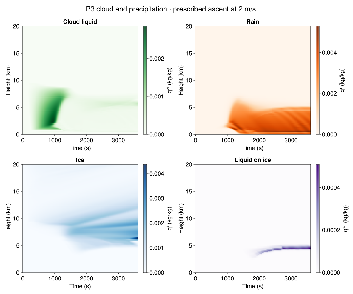
[ Info: t = 10 minutes, max cloud = 1.59e-03, rain = 1.16e-05, ice = 4.26e-04 kg/kg
[ Info: t = 20 minutes, max cloud = 1.89e-03, rain = 4.72e-03, ice = 1.27e-03 kg/kg
[ Info: t = 30 minutes, max cloud = 2.41e-04, rain = 3.97e-03, ice = 1.92e-03 kg/kg
[ Info: t = 40 minutes, max cloud = 4.15e-04, rain = 4.70e-03, ice = 2.06e-03 kg/kg
[ Info: t = 50 minutes, max cloud = 5.09e-04, rain = 4.85e-03, ice = 2.30e-03 kg/kg
[ Info: Simulation is stopping after running for 1.220 minutes.
[ Info: Simulation time 1 hour equals or exceeds stop time 1 hour.
[ Info: t = 1 hour, max cloud = 6.77e-04, rain = 5.09e-03, ice = 4.37e-03 kg/kg

Cloud and precipitation through time

Each panel shows the full time history of one condensate. Color scales are labeled separately because cloud, rain, ice, and liquid coating can have very different abundances. All mass fractions retain their model units of kg/kg. Figures are saved as high-resolution PNGs and zoomable SVGs.

qᶜˡts = FieldTimeSeries(filename, "qᶜˡ")qʳts = FieldTimeSeries(filename, "qʳ")qⁱts = FieldTimeSeries(filename, "qⁱ")qʷⁱts = FieldTimeSeries(filename, "qʷⁱ")Tts = FieldTimeSeries(filename, "T")qᵛts = FieldTimeSeries(filename, "qᵛ")δqᵛ⁺ˡts = FieldTimeSeries(filename, "δqᵛ⁺ˡ")diagnosed_δqᵛ⁺ˡts = FieldTimeSeries(filename, "diagnosed_δqᵛ⁺ˡ")

The time series is indexed over the physical column cells, excluding halos.

function plot_time_height!(layout, field_ts; title, label, colormap,                           colorbar_ticks=Makie.automatic, kwargs...)    z = znodes(field_ts.grid, Center()) / kilometers    data = permutedims(Array(field_ts[1, 1, 1:Nz, :]))    ax = Axis(layout[1, 1]; xlabel="Time (s)", ylabel="Height (km)", title)    plot = heatmap!(ax, field_ts.times, z, data; colormap, rasterize=2, kwargs...)    Colorbar(layout[1, 2], plot; label, ticks=colorbar_ticks)    return axendset_theme!(fontsize=20, linewidth=3)condensate_figure = Figure(size=(1200, 1000))Label(condensate_figure[0, 1:2], "P3 cloud and precipitation · prescribed ascent at 2 m/s"; fontsize=24)plot_time_height!(condensate_figure[1, 1], qᶜˡts;                  title = "Cloud liquid", label = "qᶜˡ (kg/kg)", colormap = :Greens)plot_time_height!(condensate_figure[1, 2], qʳts;                  title = "Rain", label = "qʳ (kg/kg)", colormap = :Oranges)plot_time_height!(condensate_figure[2, 1], qⁱts;                  title = "Ice", label = "qⁱ (kg/kg)", colormap = :Blues)plot_time_height!(condensate_figure[2, 2], qʷⁱts;                  title = "Liquid on ice", label = "qʷⁱ (kg/kg)", colormap = :Purples)save("kinematic_driver_p3_condensate.png", condensate_figure; px_per_unit=2)save("kinematic_driver_p3_condensate.svg", condensate_figure)condensate_figure

Download the condensate figure as SVG.

Temperature, vapor, and vapor excess

The two vapor-excess panels share a symmetric logarithmic color scale, linear within ±10⁻⁵ kg/kg. This resolves small vapor excesses and larger deficits on the same scale. The prognostic and diagnosed values can differ while transport, cooling, and microphysical relaxation act.

vapor_excess_limit = max(maximum(abs, δqᵛ⁺ˡts[1, 1, 1:Nz, :]),                            maximum(abs, diagnosed_δqᵛ⁺ˡts[1, 1, 1:Nz, :]))vapor_excess_colors = (; colormap = :balance,                            colorscale = Makie.Symlog10(1e-5),                            colorrange = (-vapor_excess_limit, vapor_excess_limit),                            colorbar_ticks = ([-1e-3, -1e-4, 0, 1e-4, 1e-3],                                              ["−10⁻³", "−10⁻⁴", "0", "10⁻⁴", "10⁻³"]))thermodynamics_figure = Figure(size=(1200, 1000))plot_time_height!(thermodynamics_figure[1, 1], Tts;                  title = "Temperature", label = "T (K)", colormap = :thermal)plot_time_height!(thermodynamics_figure[1, 2], qᵛts;                  title = "Water vapor", label = "qᵛ (kg/kg)", colormap = :Blues)plot_time_height!(thermodynamics_figure[2, 1], δqᵛ⁺ˡts;                  title = "Prognostic vapor excess", label = "δqᵛ⁺ˡ (kg/kg)", vapor_excess_colors...)plot_time_height!(thermodynamics_figure[2, 2], diagnosed_δqᵛ⁺ˡts;                  title = "Diagnosed vapor excess", label = "qᵛ − qᵛ⁺ˡ (kg/kg)", vapor_excess_colors...)save("kinematic_driver_p3_thermodynamics.png", thermodynamics_figure; px_per_unit=2)save("kinematic_driver_p3_thermodynamics.svg", thermodynamics_figure)thermodynamics_figure

Download the thermodynamics figure as SVG.

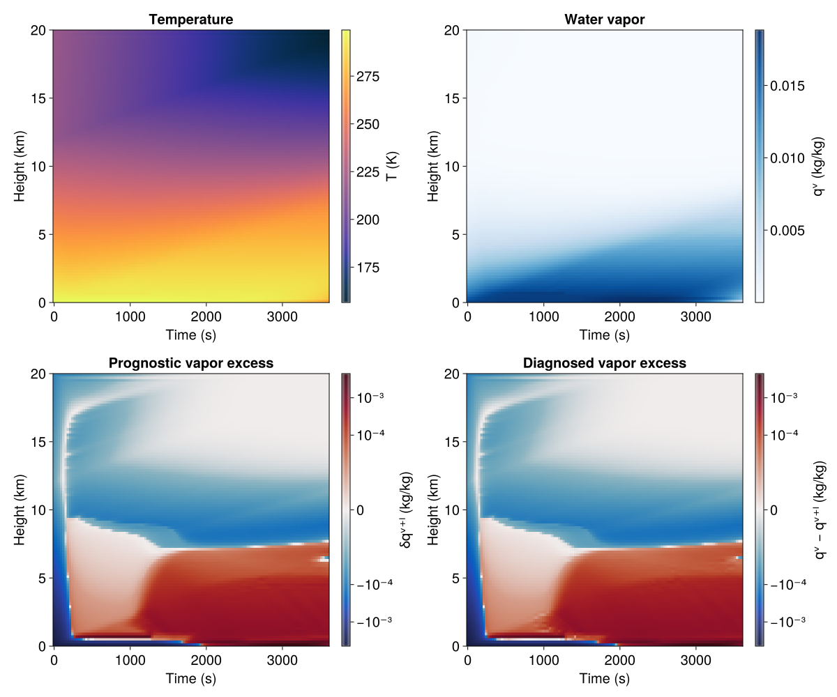
Unlike a closed parcel, the column's water inventory changes through inflow, outflow, sedimentation, and the prescribed divergence correction. A quantitative comparison with another kinematic driver must match those terms as well as the sounding, velocity profile, P3 options, and numerical resolution.

Julia version and environment information

This example was executed with the following version of Julia:

using InteractiveUtils: versioninfoversioninfo()

Julia Version 1.13.2
Commit 45b6d15e34b (2026-10-14 20:33 UTC)
Build Info:
  Official https://julialang.org release
Platform Info:
  OS: Linux (x86_64-linux-gnu)
  CPU: 8 × AMD EPYC 7R13 Processor
  WORD_SIZE: 64
  LLVM: libLLVM-20.1.8 (ORCJIT, znver3)
  GC: Built with stock GC
Threads: 1 default, 1 interactive, 5 GC (on 8 virtual cores)
Environment:
  JULIA_NUM_GC_THREADS = 4,1
  JULIA_GPG = 64B779A570972FFF7BFC2B54EAD471E1A1F2C10A
  JULIA_LOAD_PATH = :@breeze
  JULIA_PKG_SERVER_REGISTRY_PREFERENCE = eager
  JULIA_VERSION = 1.13.2
  JULIA_DEPOT_PATH = /usr/local/share/julia:
  JULIA_PATH = /usr/local/julia
  JULIA_PROJECT = @breeze

These were the top-level packages installed in the environment:

import PkgPkg.status()

Status `/__w/Breeze.jl/Breeze.jl/docs/Project.toml`
⌃ [86bc3604] AtmosphericProfilesLibrary v0.1.8
  [660aa2fb] Breeze v0.15.1 `.`
⌃ [052768ef] CUDA v6.4.1
  [13f3f980] CairoMakie v0.15.17
  [6a9e3e04] CloudMicrophysics v0.49.1
  [e30172f5] Documenter v1.20.0
  [daee34ce] DocumenterCitations v1.5.0
  [b6400b83] DocumenterCodeBlocks v1.5.1
  [1c52b33b] DocumenterLandingPage v0.2.2
  [7da242da] Enzyme v0.13.219
⌅ [46192b85] GPUArraysCore v0.2.1
⌅ [63c18a36] KernelAbstractions v0.9.47
  [98b081ad] Literate v2.21.1
  [85f8d34a] NCDatasets v0.14.15
  [cd8119b0] NumericalRadiation v0.2.1
  [9e8cae18] Oceananigans v0.118.1
  [a01a1ee8] RRTMGP v1.1.1
  [3c362404] Reactant v0.2.308
  [276daf66] SpecialFunctions v2.9.2
  [10745b16] Statistics v1.11.5
  [b77e0a4c] InteractiveUtils v1.11.0
  [44cfe95a] Pkg v1.13.0
  [9a3f8284] Random v1.11.0
Info Packages marked with ⌃ and ⌅ have new versions available. Those with ⌃ may be upgradable, but those with ⌅ are restricted by compatibility constraints from upgrading. To see why use `status --outdated`

This page was generated using Literate.jl.