Near-global ocean simulation

This example sets up and runs a near-global ocean simulation using the Oceananigans.jl and NumericalEarth.jl. The simulation covers latitudes from 75°S to 75°N, with a horizontal resolution of 1/4 degree and 40 vertical levels.

The simulation's results are visualized with the CairoMakie.jl package.

Initial setup with package imports

We begin by importing the necessary Julia packages for visualization (CairoMakie), ocean modeling (Oceananigans, NumericalEarth), handling dates and times (CFTime, Dates), and CUDA for running on CUDA-enabled GPUs. These packages provide the foundational tools for setting up the simulation environment, including grid setup, physical processes modeling, and data visualization.

using NumericalEarth
using Oceananigans
using Oceananigans.Units
using CairoMakie
using CFTime
using Dates
using Printf
using CUDA

[ Info: Oceananigans will use 8 threads

Grid configuration

We define a global grid with a horizontal resolution of 1/4 degree and 40 vertical levels. The grid is a LatitudeLongitudeGrid spanning latitudes from 75°S to 75°N. We use an exponential vertical spacing to better resolve the upper-ocean layers. The total depth of the domain is set to 6000 meters. Finally, we specify the architecture for the simulation, which in this case is a GPU.

arch = GPU()
Nx = 1440
Ny = 600
Nz = 40

depth = 6000meters
z = ExponentialDiscretization(Nz, -depth, 0, mutable=true)

grid = LatitudeLongitudeGrid(arch;
                             size = (Nx, Ny, Nz),
                             halo = (7, 7, 7),
                             z,
                             latitude  = (-75, 75),
                             longitude = (0, 360))

1440×600×40 LatitudeLongitudeGrid{Float64, Oceananigans.Grids.Periodic, Oceananigans.Grids.Bounded, Oceananigans.Grids.Bounded} on CUDAGPU with 7×7×7 halo
├── longitude: Periodic λ ∈ [0.0, 360.0)   regularly spaced with Δλ=0.25
├── latitude:  Bounded  φ ∈ [-75.0, 75.0]  regularly spaced with Δφ=0.25
└── z:         Bounded  z ∈ [-6000.0, 0.0] variably and mutably spaced with min(Δr)=5.4194, max(Δr)=709.801

Bathymetry and immersed boundary

We use regrid_bathymetry to derive the bottom height from ETOPO1 data. To smooth the interpolated data we use 5 interpolation passes. We also fill in

• all the minor enclosed basins except the 3 largest major_basins, as well as
• regions that are shallower than minimum_depth.

bottom_height = regrid_bathymetry(grid;
                                  minimum_depth = 10meters,
                                  interpolation_passes = 5,
                                  major_basins = 3)

grid = ImmersedBoundaryGrid(grid, GridFittedBottom(bottom_height); active_cells_map=true)

1440×600×40 ImmersedBoundaryGrid{Float64, Oceananigans.Grids.Periodic, Oceananigans.Grids.Bounded, Oceananigans.Grids.Bounded} on CUDAGPU with 7×7×7 halo:
├── immersed_boundary: GridFittedBottom(mean(z)=-2513.81, min(z)=-6000.0, max(z)=0.0)
├── underlying_grid: 1440×600×40 LatitudeLongitudeGrid{Float64, Oceananigans.Grids.Periodic, Oceananigans.Grids.Bounded, Oceananigans.Grids.Bounded} on CUDAGPU with 7×7×7 halo
├── longitude: Periodic λ ∈ [0.0, 360.0)   regularly spaced with Δλ=0.25
├── latitude:  Bounded  φ ∈ [-75.0, 75.0]  regularly spaced with Δφ=0.25
└── z:         Bounded  z ∈ [-6000.0, 0.0] variably and mutably spaced with min(Δr)=5.4194, max(Δr)=709.801

Let's see what the bathymetry looks like:

h = grid.immersed_boundary.bottom_height

fig, ax, hm = heatmap(h, colormap=:deep, colorrange=(-depth, 0))
Colorbar(fig[0, 1], hm, label="Bottom height (m)", vertical=false)
save("bathymetry.png", fig)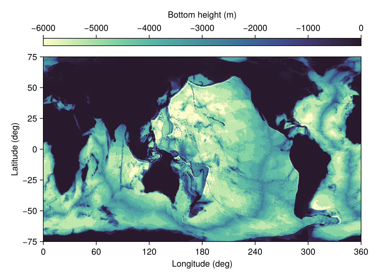

Ocean model configuration

We build our ocean model using ocean_simulation,

ocean = ocean_simulation(grid)

Simulation of HydrostaticFreeSurfaceModel{CUDAGPU, ImmersedBoundaryGrid}(time = 0 seconds, iteration = 0)
├── Next time step: 13.304 minutes
├── run_wall_time: 0 seconds
├── run_wall_time / iteration: NaN days
├── stop_time: Inf days
├── stop_iteration: Inf
├── wall_time_limit: Inf
├── minimum_relative_step: 0.0
├── callbacks: OrderedDict with 4 entries:
│   ├── stop_time_exceeded => Callback of stop_time_exceeded on IterationInterval(1)
│   ├── stop_iteration_exceeded => Callback of stop_iteration_exceeded on IterationInterval(1)
│   ├── wall_time_limit_exceeded => Callback of wall_time_limit_exceeded on IterationInterval(1)
│   └── nan_checker => Callback of NaNChecker for u on IterationInterval(100)
└── output_writers: OrderedDict with no entries

which uses the default ocean.model,

ocean.model

HydrostaticFreeSurfaceModel{CUDAGPU, ImmersedBoundaryGrid}(time = 0 seconds, iteration = 0)
├── grid: 1440×600×40 ImmersedBoundaryGrid{Float64, Oceananigans.Grids.Periodic, Oceananigans.Grids.Bounded, Oceananigans.Grids.Bounded} on CUDAGPU with 7×7×7 halo
├── timestepper: SplitRungeKuttaTimeStepper
├── tracers: (T, S, e)
├── closure: CATKEVerticalDiffusivity{VerticallyImplicitTimeDiscretization}
├── buoyancy: SeawaterBuoyancy with g=9.80665 and BoussinesqEquationOfState{Float64} with ĝ = NegativeZDirection()
├── free surface: Oceananigans.Models.HydrostaticFreeSurfaceModels.SplitExplicitFreeSurfaces.SplitExplicitFreeSurface with gravitational acceleration 9.80665 m s⁻²
│   └── substepping: FixedTimeStepSize(20.254 seconds)
├── advection scheme: 
│   ├── momentum: WENOVectorInvariant{5, Float64}(vorticity_order=9, vertical_order=5)
│   ├── T: WENO{4, Float64, Oceananigans.Utils.BackendOptimizedDivision}(order=7)
│   ├── S: WENO{4, Float64, Oceananigans.Utils.BackendOptimizedDivision}(order=7)
│   └── e: Nothing
├── vertical_coordinate: ZStarCoordinate
└── coriolis: Oceananigans.Coriolis.HydrostaticSphericalCoriolis{Oceananigans.Advection.EnstrophyConserving{Float64}, Float64, Oceananigans.Coriolis.HydrostaticFormulation}

We initialize the ocean model with ECCO4 temperature and salinity for January 1, 1992.

date = DateTime(1992, 1, 1)
set!(ocean.model, MetadataSet(:temperature, :salinity; dataset=ECCO4Monthly(), date))

Prescribed atmosphere and radiation

Next we build a prescribed atmosphere state and radiation component, which together drive the ocean simulation. The atmospheric data and downwelling shortwave / longwave radiation are both prescribed using JRA55.

atmosphere = JRA55PrescribedAtmosphere(arch)
radiation  = JRA55PrescribedRadiation(arch)
land       = JRA55PrescribedLand(arch)

1440×720×1×365 PrescribedLand on Oceananigans.Grids.LatitudeLongitudeGrid:
├── times: 365-element StepRangeLen{Float64, Base.TwicePrecision{Float64}, Base.TwicePrecision{Float64}, Int64}
└── freshwater_flux: (:rivers, :icebergs)

The coupled simulation

Next we assemble the ocean, atmosphere, and radiation into a coupled model,

coupled_model = OceanOnlyModel(ocean; atmosphere, land, radiation)

EarthSystemModel{GPU}(time = 0 seconds, iteration = 0)
├── radiation: 640×320×1×2920 PrescribedRadiation
├── atmosphere: 640×320×1×2920 PrescribedAtmosphere{Float32}
├── land: 1440×720×1×365 PrescribedLand
├── sea_ice: NumericalEarth.SeaIces.FreezingLimitedOceanTemperature{ClimaSeaIce.SeaIceThermodynamics.LinearLiquidus{Float64}}
├── ocean: HydrostaticFreeSurfaceModel{CUDAGPU, ImmersedBoundaryGrid}(time = 0 seconds, iteration = 0)
└── interfaces: ComponentInterfaces

We then create a coupled simulation.

simulation = Simulation(coupled_model; Δt=25minutes, stop_time=60days)

Simulation of EarthSystemModel{GPU}(time = 0 seconds, iteration = 0)
├── Next time step: 25 minutes
├── run_wall_time: 0 seconds
├── run_wall_time / iteration: NaN days
├── stop_time: 60 days
├── stop_iteration: Inf
├── wall_time_limit: Inf
├── minimum_relative_step: 0.0
├── callbacks: OrderedDict with 4 entries:
│   ├── stop_time_exceeded => Callback of stop_time_exceeded on IterationInterval(1)
│   ├── stop_iteration_exceeded => Callback of stop_iteration_exceeded on IterationInterval(1)
│   ├── wall_time_limit_exceeded => Callback of wall_time_limit_exceeded on IterationInterval(1)
│   └── nan_checker => Callback of NaNChecker for T_ocean on IterationInterval(100)
└── output_writers: OrderedDict with no entries

We define a callback function to monitor the simulation's progress,

wall_time = Ref(time_ns())

function progress(sim)
    ocean = sim.model.ocean
    u, v, w = ocean.model.velocities
    T = ocean.model.tracers.T

    Tmax = maximum(interior(T))
    Tmin = minimum(interior(T))

    umax = (maximum(abs, interior(u)),
            maximum(abs, interior(v)),
            maximum(abs, interior(w)))

    step_time = 1e-9 * (time_ns() - wall_time[])

    msg = @sprintf("Iter: %d, time: %s, Δt: %s", iteration(sim), prettytime(sim), prettytime(sim.Δt))
    msg *= @sprintf(", max|u|: (%.2e, %.2e, %.2e) m s⁻¹, extrema(T): (%.2f, %.2f) ᵒC, wall time: %s",
                    umax..., Tmax, Tmin, prettytime(step_time))

    @info msg

    wall_time[] = time_ns()
end

simulation.callbacks[:progress] = Callback(progress, TimeInterval(5days))

Callback of progress on TimeInterval(5 days)

Set up output writers

We define output writers to save the simulation data at regular intervals. In this case, we save the surface fluxes and surface fields at a relatively high frequency (every day). The indices keyword argument allows us to save only a slice of the three dimensional variable. Below, we use indices to save only the values of the variables at the surface, which corresponds to k = grid.Nz

outputs = merge(ocean.model.tracers, ocean.model.velocities)
ocean.output_writers[:surface] = JLD2Writer(ocean.model, outputs;
                                            schedule = TimeInterval(1days),
                                            including = [:grid],
                                            filename = "near_global_surface_fields",
                                            indices = (:, :, grid.Nz),
                                            with_halos = true,
                                            overwrite_existing = true,
                                            array_type = Array{Float32})

JLD2Writer scheduled on TimeInterval(1 day):
├── filepath: near_global_surface_fields.jld2
├── 6 outputs: (T, S, e, u, v, w)
├── array_type: Array{Float32}
├── including: [:grid]
├── file_splitting: NoFileSplitting
└── file size: 0 bytes (file not yet created)

Running the simulation

run!(simulation)

[ Info: Initializing simulation...
[ Info: Iter: 0, time: 0 seconds, Δt: 25 minutes, max|u|: (0.00e+00, 0.00e+00, 0.00e+00) m s⁻¹, extrema(T): (31.53, -1.88) ᵒC, wall time: 2.561 minutes
[ Info:     ... simulation initialization complete (7.918 seconds)
[ Info: Executing initial time step...
┌ Warning: error ArgumentError("a group or dataset named grid is already present within this group") thrown when trying to serialize the grid at serialized/grid
└ @ Oceananigans.OutputWriters /storage5/github-action-runners/julia-depot/packages/Oceananigans/pztwa/src/OutputWriters/jld2_writer.jl:234
[ Info:     ... initial time step complete (3.341 minutes).
[ Info: Iter: 288, time: 5 days, Δt: 25 minutes, max|u|: (2.40e+00, 2.20e+00, 2.29e-02) m s⁻¹, extrema(T): (32.60, -1.92) ᵒC, wall time: 6.472 minutes
[ Info: Iter: 576, time: 10 days, Δt: 25 minutes, max|u|: (1.96e+00, 2.32e+00, 1.41e-02) m s⁻¹, extrema(T): (33.63, -2.17) ᵒC, wall time: 3.230 minutes
[ Info: Iter: 864, time: 15 days, Δt: 25 minutes, max|u|: (2.23e+00, 2.34e+00, 1.43e-02) m s⁻¹, extrema(T): (33.62, -2.42) ᵒC, wall time: 3.238 minutes
[ Info: Iter: 1152, time: 20 days, Δt: 25 minutes, max|u|: (2.28e+00, 2.22e+00, 1.20e-02) m s⁻¹, extrema(T): (34.32, -2.10) ᵒC, wall time: 3.237 minutes
[ Info: Iter: 1440, time: 25 days, Δt: 25 minutes, max|u|: (2.34e+00, 2.30e+00, 1.59e-02) m s⁻¹, extrema(T): (34.38, -2.01) ᵒC, wall time: 3.239 minutes
[ Info: Iter: 1728, time: 30 days, Δt: 25 minutes, max|u|: (4.18e+00, 2.61e+00, 3.06e-02) m s⁻¹, extrema(T): (34.75, -2.26) ᵒC, wall time: 3.235 minutes
[ Info: Iter: 2016, time: 35 days, Δt: 25 minutes, max|u|: (2.09e+00, 2.52e+00, 4.15e-02) m s⁻¹, extrema(T): (34.44, -2.23) ᵒC, wall time: 3.234 minutes
[ Info: Iter: 2304, time: 40 days, Δt: 25 minutes, max|u|: (3.39e+00, 3.03e+00, 2.97e-02) m s⁻¹, extrema(T): (34.72, -2.19) ᵒC, wall time: 3.242 minutes
[ Info: Iter: 2592, time: 45 days, Δt: 25 minutes, max|u|: (2.70e+00, 2.50e+00, 2.82e-02) m s⁻¹, extrema(T): (35.06, -2.21) ᵒC, wall time: 3.231 minutes
[ Info: Iter: 2880, time: 50 days, Δt: 25 minutes, max|u|: (2.18e+00, 2.56e+00, 2.92e-02) m s⁻¹, extrema(T): (34.41, -2.21) ᵒC, wall time: 3.246 minutes
[ Info: Iter: 3168, time: 55 days, Δt: 25 minutes, max|u|: (4.28e+00, 3.45e+00, 3.02e-02) m s⁻¹, extrema(T): (34.12, -2.21) ᵒC, wall time: 3.238 minutes
[ Info: Simulation is stopping after running for 42.178 minutes.
[ Info: Simulation time 60 days equals or exceeds stop time 60 days.
[ Info: Iter: 3456, time: 60 days, Δt: 25 minutes, max|u|: (1.92e+00, 1.85e+00, 2.79e-02) m s⁻¹, extrema(T): (34.25, -2.18) ᵒC, wall time: 3.238 minutes

A pretty movie

It's time to make a pretty movie of the simulation. First we load the output we've been saving on disk and plot the final snapshot:

u = FieldTimeSeries("near_global_surface_fields.jld2", "u"; backend = OnDisk())
v = FieldTimeSeries("near_global_surface_fields.jld2", "v"; backend = OnDisk())
T = FieldTimeSeries("near_global_surface_fields.jld2", "T"; backend = OnDisk())
e = FieldTimeSeries("near_global_surface_fields.jld2", "e"; backend = OnDisk())

times = u.times
Nt = length(times)

n = Observable(Nt)

land = interior(T.grid.immersed_boundary.bottom_height) .>= 0

Tn = @lift begin
    Tn = interior(T[$n])
    Tn[land] .= NaN
    view(Tn, :, :, 1)
end

en = @lift begin
    en = interior(e[$n])
    en[land] .= NaN
    view(en, :, :, 1)
end

un = Field{Face, Center, Nothing}(u.grid)
vn = Field{Center, Face, Nothing}(v.grid)

s = @at (Center, Center, Nothing) sqrt(un^2 + vn^2) # compute √(u²+v²) and interpolate back to Center, Center
s = Field(s)

sn = @lift begin
    parent(un) .= parent(u[$n])
    parent(vn) .= parent(v[$n])
    compute!(s)
    sn = interior(s)
    sn[land] .= NaN
    view(sn, :, :, 1)
end

title = @lift string("Near-global 1/4 degree ocean simulation after ",
                     prettytime(times[$n] - times[1]))

λ, φ, _ = nodes(T) # T, e, and s all live on the same grid locations

fig = Figure(size = (1000, 1500))

axs = Axis(fig[1, 1], xlabel="Longitude (deg)", ylabel="Latitude (deg)")
axT = Axis(fig[2, 1], xlabel="Longitude (deg)", ylabel="Latitude (deg)")
axe = Axis(fig[3, 1], xlabel="Longitude (deg)", ylabel="Latitude (deg)")

hm = heatmap!(axs, λ, φ, sn, colorrange = (0, 0.5), colormap = :deep, nan_color=:lightgray)
Colorbar(fig[1, 2], hm, label = "Surface Speed (m s⁻¹)")

hm = heatmap!(axT, λ, φ, Tn, colorrange = (-1, 30), colormap = :magma, nan_color=:lightgray)
Colorbar(fig[2, 2], hm, label = "Surface Temperature (ᵒC)")

hm = heatmap!(axe, λ, φ, en, colorrange = (0, 1e-3), colormap = :solar, nan_color=:lightgray)
Colorbar(fig[3, 2], hm, label = "Turbulent Kinetic Energy (m² s⁻²)")

Label(fig[0, :], title)

save("snapshot.png", fig)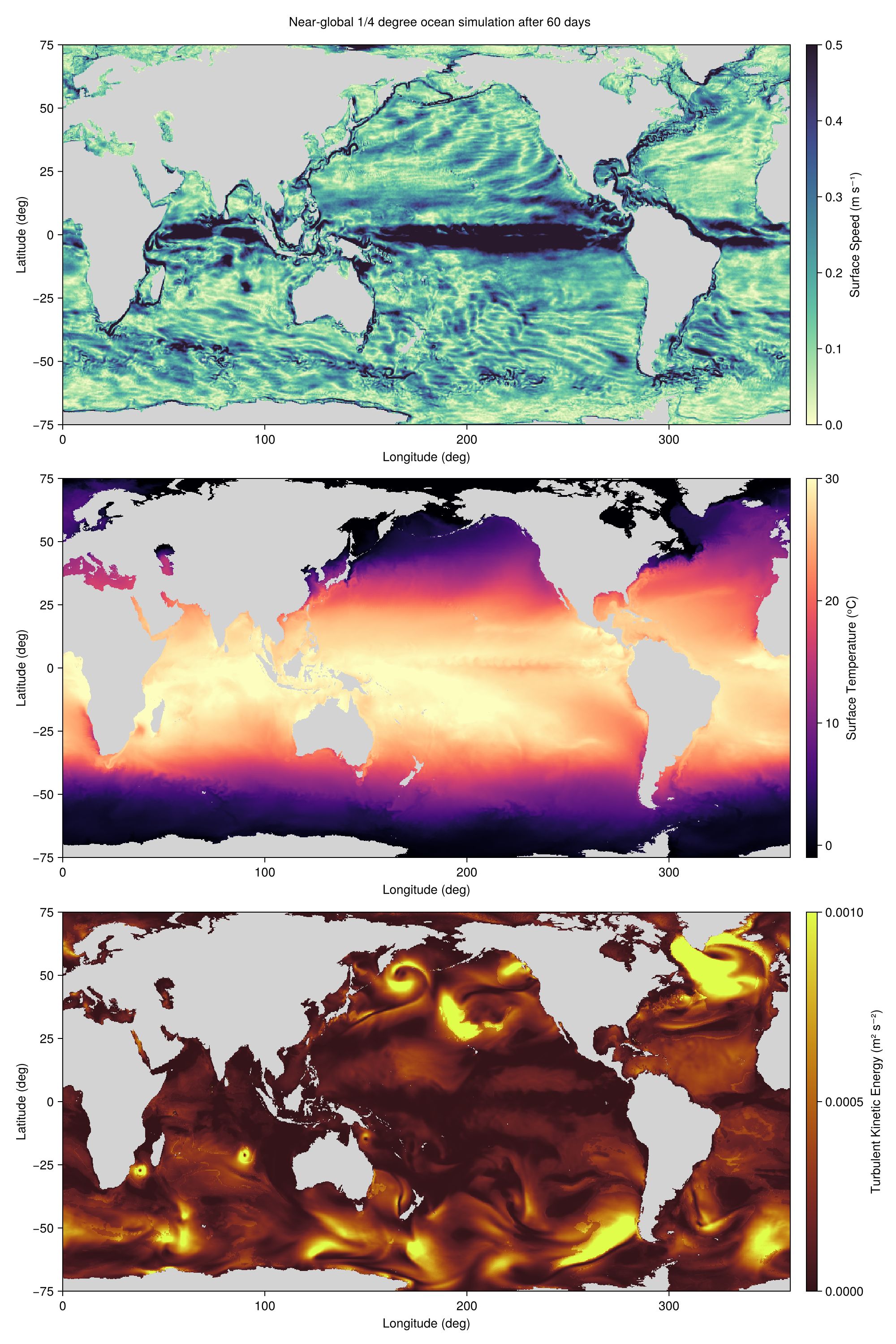

And now we make a movie:

CairoMakie.record(fig, "near_global_ocean_surface.mp4", 1:Nt, framerate = 8) do nn
    n[] = nn
end

This page was generated using Literate.jl.