CO₂ forcing with ecCKD

This example computes the instantaneous, clear-sky longwave effect of doubling CO₂ — the reduction in outgoing longwave radiation (OLR) at the top of the atmosphere when the CO₂ column amount is doubled with temperature, humidity, and everything else held fixed — using an reference ecCKD gas-optics model, i.e. the full tabulated g-point machinery a host model would run. The longwave page computes the same class of benchmark with the analytic-band Williams scheme; the two pages pose a related CO₂-doubling question through two different gas-optics and solver interfaces.

We build one idealized clear-sky column and solve its longwave fluxes at two CO₂ concentrations through a small helper.

using NumericalRadiation
using NCDatasets
using Printf

gas_optics = read_reference_ecckd_gas_optics("32x32"; names=(:composite, :h2o, :co2))

The column: $Nz$ layers with interface pressures $pᵢ$ (Pa, top of atmosphere first), layer pressures $p$ at their midpoints, and the dry-air molar amount $nᵈ$ of each layer from the hydrostatic relation:

constants = PhysicalConstants()
g  = constants.gravity               # m s⁻²
mᵈ = constants.dry_air_molar_mass    # kg mol⁻¹

Nz = 48
pᵢ = collect(range(2_000, 101_325; length=Nz + 1))
p  = 0.5 .* (pᵢ[1:end-1] .+ pᵢ[2:end])
nᵈ = diff(pᵢ) ./ (g * mᵈ)                                # mol m⁻²

Tˢ = 300
T  = clamp.(Tˢ .- 65 .* (1 .- (p ./ 101_325) .^ 0.286), 200, Tˢ)
Tᵢ = clamp.(Tˢ .- 65 .* (1 .- (pᵢ ./ 101_325) .^ 0.286), 200, Tˢ)

The temperature profile is an idealized lapse rate capped at 200 K aloft; it is prescribed and does not respond to the radiation.

function solve_column(χCO₂)
    atmosphere = ColumnAtmosphere(;
        pressure_layers = p,
        pressure_interfaces = pᵢ,
        temperature_layers = T,
        temperature_interfaces = Tᵢ,
        gases = (composite = nᵈ,
                 h2o = 0.006 .* nᵈ,
                 co2 = χCO₂ .* nᵈ),
        surface = (temperature=Tˢ,),
        geometry = (cos_zenith=0.5,),
        constants)

    Ngˡʷ = length(gas_optics.longwave_weights)
    Ngˢʷ = length(gas_optics.shortwave_weights)
    longwave = LongwaveOptics(zeros(Ngˡʷ, Nz), zeros(Ngˡʷ, Nz);
                              source_top = zeros(Ngˡʷ, Nz),
                              source_bottom = zeros(Ngˡʷ, Nz),
                              weights = zeros(Ngˡʷ))
    shortwave = ShortwaveOptics(zeros(Ngˢʷ, Nz); weights=zeros(Ngˢʷ))
    fluxes = RadiativeFluxes(longwave_up = zeros(Nz + 1),
                             longwave_down = zeros(Nz + 1),
                             shortwave_up = zeros(Nz + 1),
                             shortwave_down = zeros(Nz + 1))

    optical_properties!(longwave, shortwave, gas_optics, atmosphere)
    surface_emission = surface_longwave_emission(gas_optics, Tˢ)
    radiative_fluxes!(fluxes, CloudlessLongwave(), longwave, atmosphere,
                      LongwaveBoundaryConditions(surface_longwave_up=surface_emission))
    return (; olr=fluxes.longwave_up[1], up=fluxes.longwave_up)
end

Solve the same column at present-day and doubled CO₂:

base = solve_column(420e-6)
doubled = solve_column(840e-6)

Sign convention: the instantaneous forcing is the reduction in OLR, base-CO₂ OLR minus doubled-CO₂ OLR, so a positive value means the doubled column emits less to space.

ΔOLR = base.olr - doubled.olr

@printf("OLR at 420 ppm CO₂:                        %6.2f W m⁻²\n", base.olr)
@printf("OLR at 840 ppm CO₂:                        %6.2f W m⁻²\n", doubled.olr)
@printf("instantaneous clear-sky LW ΔOLR (2×CO₂):   %6.2f W m⁻²\n", ΔOLR)

OLR at 420 ppm CO₂:                        348.23 W m⁻²
OLR at 840 ppm CO₂:                        345.84 W m⁻²
instantaneous clear-sky LW ΔOLR (2×CO₂):     2.39 W m⁻²

Doubling CO₂ reduces the OLR of this fixed column by a few W m⁻². The upwelling-flux profiles show how that reduction varies with height:

using CairoMakie

fig = Figure(size=(760, 440))

pressure_ticks = [20, 50, 100, 200, 300, 500, 700, 1000]

ax1 = Axis(fig[1, 1]; xlabel = "Upwelling longwave flux (W m⁻²)",
           ylabel = "Pressure (hPa)", yscale = log10, yreversed = true,
           yticks = (pressure_ticks, string.(pressure_ticks)),
           title = "Upwelling longwave flux")
lines!(ax1, base.up, pᵢ ./ 100; color=:steelblue4, linewidth=2, label="420 ppm")
lines!(ax1, doubled.up, pᵢ ./ 100; color=:firebrick, linewidth=2, label="840 ppm")
axislegend(ax1; position=:rt, framevisible=false)

ax2 = Axis(fig[1, 2]; xlabel = "Δ upwelling flux, 1× − 2× (W m⁻²)",
           ylabel = "Pressure (hPa)", yscale = log10, yreversed = true,
           yticks = (pressure_ticks, string.(pressure_ticks)),
           title = "OLR reduction from doubling CO₂")
vlines!(ax2, [0]; color=(:black, 0.4), linestyle=:dash)
lines!(ax2, base.up .- doubled.up, pᵢ ./ 100; color=:firebrick, linewidth=2)
scatter!(ax2, [ΔOLR], [pᵢ[1] / 100]; color=:firebrick, markersize=10)
text!(ax2, ΔOLR, pᵢ[1] / 100;
      text = "TOA: $(round(ΔOLR; digits = 2)) W m⁻² ",
      align = (:right, :top), offset = (-6, 0), fontsize = 12)

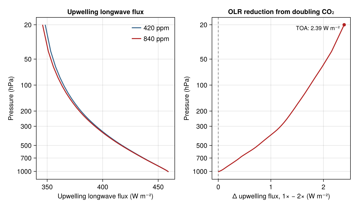
The difference panel is the measurement itself. At the surface the difference is zero by construction (the upwelling boundary flux is prescribed); it departs from zero within the atmosphere and reaches the reported TOA value annotated above — the instantaneous clear-sky forcing printed earlier. Temperatures are prescribed in this column, so this is a statement about radiative transfer through a fixed state, not about the temperature response that such a forcing would eventually drive.

This page was generated using Literate.jl.