Correlated-k model spread: clear-sky longwave
Every correlated-k radiation model makes a k-reduction choice: how many g points, what band structure, which training data. This example runs a small family of such models on one clear-sky column defined once physically and shows the spread of their longwave fluxes and heating rates. The family is the ecCKD 32-g-point FSCK model, the ecCKD 64-g-point narrow-band model, and RRTMGP (256 g points, through the package's NumericalRadiationRRTMGPExt adapter) — three members of one model class on equal footing. Nothing here ranks a model or measures error against a truth; the spread itself is the message — a measured correlated-k implementation spread on this column.
One physical column, two gas representations
The shared definition is the physical state: pressures, temperatures, and per-gas dry-air volume mixing ratios $χ$ (RRTMGP's native convention, established by its compute_col_gas_kernel!). RRTMGP consumes the mixing ratios directly; the ecCKD path consumes layer molar amounts in mol m⁻², so the conversion between the two representations is written out explicitly below and cross-checked against RRTMGP's own column computation.
using NumericalRadiation
using NCDatasets     # NetCDF reader extension (ecCKD files)
using ClimaComms     # RRTMGP adapter extension trigger …
using RRTMGP         # … and RRTMGP itself
using Printf
The column: $Nz$ layers with interface pressures $pᵢ$ (Pa, top of atmosphere first), layer pressures $p$, an idealized capped lapse rate, and analytic moisture and ozone mixing-ratio profiles:
Nz = 48
pᵢ = collect(range(2_000, 101_325; length=Nz + 1))
p  = 0.5 .* (pᵢ[1:end-1] .+ pᵢ[2:end])

Tˢ = 300
T  = clamp.(Tˢ .- 65 .* (1 .- (p ./ 101_325) .^ 0.286), 200, Tˢ)
Tᵢ = clamp.(Tˢ .- 65 .* (1 .- (pᵢ ./ 101_325) .^ 0.286), 200, Tˢ)

χH₂O = @. 0.015 * (p / 101_325)^3 + 3e-6      # moist below, dry aloft
χO₃  = @. 3e-8 + 5e-6 * (2_000 / p)           # crude ozone increase aloft
χCO₂ = 420e-6
χCH₄ = 1.8e-6
χN₂O = 330e-9
The hydrostatic relation gives the dry-air molar amount $nᵈ$ of each layer. With $χ$ relative to dry air, the layer's mass per area is $nᵈ (m^d + χ_{H₂O}\, m^v)$, so (dry-air molar-mass convention, matching RRTMGP):
constants = PhysicalConstants()      # shared by both columns and the RRTMGP adapter below
g  = constants.gravity               # m s⁻²
mᵈ = constants.dry_air_molar_mass    # kg mol⁻¹
mᵛ = constants.water_molar_mass      # kg mol⁻¹

dry_air_amounts(χH₂O, pᵢ) = [(pᵢ[k + 1] - pᵢ[k]) / (g * (mᵈ + mᵛ * χH₂O[k])) for k in 1:(length(pᵢ) - 1)]

nᵈ = dry_air_amounts(χH₂O, pᵢ)                # mol m⁻²
Each representation gets its own ColumnAtmosphere. Gas-set parity needs care on the ecCKD side: the tabulated composite background contains the reference contribution of every tabulated gas, and activating a gas subtracts its reference mole fraction times the composite amount before adding the requested amount. A gas left out of names is therefore kept at its reference abundance, not removed. So the full tuple is activated here: CH₄ and N₂O carry the same abundances as the RRTMGP side, and the CFCs are activated with zero amount — which removes their reference contribution — because RRTMGP's clear-sky lookup has no CFC fields. Both surfaces emit as blackbodies.
ecckd_atmosphere = ColumnAtmosphere(;
    pressure_layers = p,
    pressure_interfaces = pᵢ,
    temperature_layers = T,
    temperature_interfaces = Tᵢ,
    gases = (composite = nᵈ,
             h2o = χH₂O .* nᵈ,
             o3 = χO₃ .* nᵈ,
             co2 = χCO₂ .* nᵈ,
             ch4 = χCH₄ .* nᵈ,
             n2o = χN₂O .* nᵈ,
             cfc11 = 0,
             cfc12 = 0),
    surface = (temperature=Tˢ,),
    geometry = (cos_zenith=0.5,),
    constants)

rrtmgp_atmosphere = ColumnAtmosphere(;
    pressure_layers = p,
    pressure_interfaces = pᵢ,
    temperature_layers = T,
    temperature_interfaces = Tᵢ,
    gases = (h2o = χH₂O, o3 = χO₃, co2 = χCO₂,
             ch4 = χCH₄, n2o = χN₂O,
             o2 = 0.20946, n2 = 0.78084, co = 0),
    surface = (temperature=Tˢ,),
    geometry = (cos_zenith=0.5,),
    constants)
The ecCKD members
Both reference longwave models — the 32-g single-band FSCK table and the 64-g narrow-band table — run through the same staged calls. The surface boundary uses each model's own per-g Planck emission via surface_longwave_emission; a scalar $σT⁴$ boundary would be spectrally gray and misplace surface emission across g points.
intended_gases = (:composite, :h2o, :o3, :co2, :ch4, :n2o, :cfc11, :cfc12)

function ecckd_member(selector)
    gas_optics = read_reference_ecckd_gas_optics(selector; names=intended_gases)
    @assert NumericalRadiation.gas_names(gas_optics) == intended_gases
    Ngˡʷ = length(gas_optics.longwave_weights)
    Ngˢʷ = length(gas_optics.shortwave_weights)
    longwave = LongwaveOptics(zeros(Ngˡʷ, Nz),
                              zeros(Ngˡʷ, Nz);
                              source_top = zeros(Ngˡʷ, Nz),
                              source_bottom = zeros(Ngˡʷ, Nz),
                              weights = zeros(Ngˡʷ))
    shortwave = ShortwaveOptics(zeros(Ngˢʷ, Nz); weights=zeros(Ngˢʷ))
    fluxes = RadiativeFluxes(longwave_up = zeros(Nz + 1),
                             longwave_down = zeros(Nz + 1),
                             shortwave_up = zeros(Nz + 1),
                             shortwave_down = zeros(Nz + 1))
    optical_properties!(longwave, shortwave, gas_optics, ecckd_atmosphere)
    surface_emission = surface_longwave_emission(gas_optics, Tˢ)
    radiative_fluxes!(fluxes, CloudlessLongwave(), longwave, ecckd_atmosphere,
                      LongwaveBoundaryConditions(surface_longwave_up=surface_emission))
    Ṫ = zeros(Nz)
    heating_rates!(Ṫ, fluxes, ecckd_atmosphere)
    return (; fluxes, Ṫ)
end
The RRTMGP member
One member of the same family, with its own k-reduction (256 longwave g points), run through the package's adapter extension. The adapter builds RRTMGP's parameters from the same constants, so both representations use one gravity and one pair of molar masses:
rrtmgp_extension = Base.get_extension(NumericalRadiation, :NumericalRadiationRRTMGPExt)

function rrtmgp_member()
    model = rrtmgp_extension.RRTMGPClearSkyModel(Float64; constants)
    boundary = rrtmgp_extension.RRTMGPBoundaryConditions(
        surface_temperature = Tˢ,
        surface_emissivity = 1,
        surface_albedo = 0,
        toa_shortwave_down = 0,   # longwave-only page
        cos_zenith = 0.5)
    workspace = radiation_workspace(model, rrtmgp_atmosphere)
    fluxes = RadiativeFluxes(longwave_up = zeros(Nz + 1),
                             longwave_down = zeros(Nz + 1),
                             shortwave_up = zeros(Nz + 1),
                             shortwave_down = zeros(Nz + 1))
    radiative_fluxes!(fluxes, model, rrtmgp_atmosphere, boundary, workspace)
    @assert all(iszero, fluxes.shortwave_up)
    @assert all(iszero, fluxes.shortwave_down)
    Ṫ = zeros(Nz)
    heating_rates!(Ṫ, fluxes, rrtmgp_atmosphere)
    return (; fluxes, Ṫ, workspace)
end

rrtmgp = rrtmgp_member()
Before using the fluxes, verify the representation bridge: the dry-air amounts computed by dry_air_amounts must equal the dry column RRTMGP itself computed from the same pressures and mixing ratios (RRTMGP stores molecules cm⁻², and its levels are bottom-up, hence the unit factor with Avogadro's number $Nᴬ$ and the index reversal):
Nᴬ = constants.avogadro_number

molecular_column_rrtmgp = reverse(rrtmgp.workspace.atmospheric_state.layerdata[1, :, 1])
molecular_column_ecckd = nᵈ .* Nᴬ ./ 1e4
relative_error = maximum(abs.(molecular_column_rrtmgp .- molecular_column_ecckd) ./ molecular_column_ecckd)
@assert relative_error < 1e-6
relative_error3.0754807242624894e-16The family, assembled
family = [(name = "ecCKD 32 (FSCK)", member = ecckd_member("32x32"),
           color = :steelblue4),
          (name = "ecCKD 64 (narrow-band)", member = ecckd_member("64x32"),
           color = :darkorange3),
          (name="RRTMGP (256 g)", member=rrtmgp, color=:firebrick)]

println("OLR by family member:")
for f in family
    @printf("  %-24s %7.2f W m⁻²\n", f.name, f.member.fluxes.longwave_up[1])
end
olr = [f.member.fluxes.longwave_up[1] for f in family]
@printf("family spread, max − min:  %7.2f W m⁻²\n", maximum(olr) - minimum(olr))
OLR by family member:
ecCKD 32 (FSCK) 380.14 W m⁻²
ecCKD 64 (narrow-band) 379.26 W m⁻²
RRTMGP (256 g) 378.01 W m⁻²
family spread, max − min: 2.14 W m⁻²
The spread, panel by panel
Left: up- and downwelling flux profiles for every member (color = model, solid = up, dashed = down). Right: the heating-rate profiles. The shared legend sits outside the axes.
using CairoMakie

fig = Figure(size=(940, 480))

pressure_ticks = [20, 50, 100, 200, 300, 500, 700, 1000]

ax1 = Axis(fig[1, 1]; xlabel = "Longwave flux (W m⁻²)",
           ylabel = "Pressure (hPa)", yscale = log10, yreversed = true,
           yticks = (pressure_ticks, string.(pressure_ticks)),
           title = "Fluxes")
for f in family
    lines!(ax1, f.member.fluxes.longwave_up, pᵢ ./ 100; color=f.color, linewidth=2)
    lines!(ax1, f.member.fluxes.longwave_down, pᵢ ./ 100; color=f.color, linewidth=2, linestyle=:dash)
end

ax2 = Axis(fig[1, 2]; xlabel = "Ṫ (K day⁻¹)",
           ylabel = "Pressure (hPa)", yscale = log10, yreversed = true,
           yticks = (pressure_ticks, string.(pressure_ticks)),
           title = "Heating rates")
vlines!(ax2, [0]; color=(:black, 0.4), linestyle=:dash)
for f in family
    lines!(ax2, f.member.Ṫ .* 86_400, p ./ 100; color=f.color, linewidth=2)
end

legend_entries = vcat(
    [LineElement(color=f.color, linewidth=2) for f in family],
    [LineElement(color=:gray30, linewidth=2, linestyle=:solid),
     LineElement(color=:gray30, linewidth=2, linestyle=:dash)])
Legend(fig[2, 1:2], legend_entries,
       vcat([f.name for f in family], ["up", "down"]);
       orientation = :horizontal, framevisible = false)
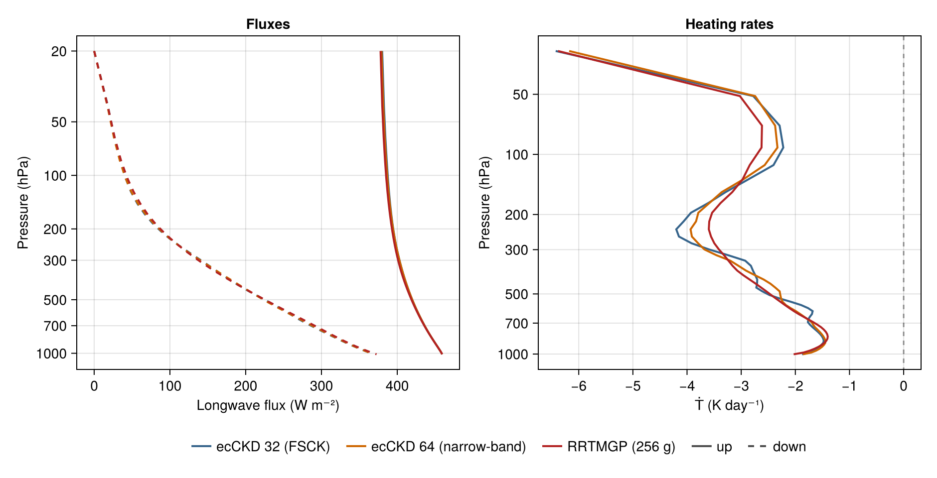
The printed table and the panels above are the result: on this one idealized clear-sky column, with matched pressures, temperatures, and treated-gas composition, the family members differ by the amounts shown. The experiment does not separate a member's gas-optics tables from its transfer implementation — each member runs both as a whole — and nothing here ranks a member or measures an error against a reference; a line-by-line benchmark would be required for that. What the spread does measure is how much choosing among these correlated-k implementations — tables, training, spectroscopy, and transfer together — moves clear-sky longwave fluxes and heating rates on this column.
This page was generated using Literate.jl.