Longwave: Williams (2026) Simple Spectral Model
The AnalyticBandLongwave solver advances Schwarzschild's two-stream equations
\[\frac{d\mathscr{I}^{\uparrow}}{d\tau} = \mathscr{I}^{\uparrow} - \pi B(T), \qquad \frac{d\mathscr{I}^{\downarrow}}{d\tau} = \pi B(T) - \mathscr{I}^{\downarrow}\]
at each of Nwavenumbers = 41 evenly spaced wavenumbers between 10 and 2500 cm⁻¹ (inclusive of both endpoints, spacing 62.25 cm⁻¹) and integrates the resulting fluxes spectrally.
Absorption spectra
The scheme represents three analytic sources of clear-sky absorption:
using NumericalRadiation
using CairoMakie

longwave = AnalyticBandLongwave(Float64)
ν̃ = range(longwave.wavenumber_min, longwave.wavenumber_max, length=500)

# Replace zeros with NaN so the log-y plot shows gaps where a band is inactive.
nan_zero(v) = [x == 0 ? NaN : x for x in v]

water_vapor_line_absorption      = nan_zero([water_vapor_line_absorption_reference(ν, longwave)      for ν in ν̃])
water_vapor_continuum_absorption =          [water_vapor_continuum_absorption_reference(ν, longwave) for ν in ν̃]
carbon_dioxide_absorption        = nan_zero([carbon_dioxide_absorption_reference(ν, longwave)        for ν in ν̃])

fig = Figure(size=(760, 440))
ax  = Axis(fig[1, 1];
           xlabel = "Wavenumber ν̃ [cm⁻¹]",
           ylabel = "κ [m² kg⁻¹]",
           yscale = log10,
           title  = "Williams (2026) reference absorption (T = 260 K, p = 500 hPa)")
lines!(ax, ν̃, water_vapor_line_absorption;      label="H₂O line",      linewidth=2)
lines!(ax, ν̃, water_vapor_continuum_absorption; label="H₂O continuum", linewidth=2)
lines!(ax, ν̃, carbon_dioxide_absorption;        label="CO₂ 15 μm",      linewidth=2, linestyle=:dash)
axislegend(ax; position=:rt)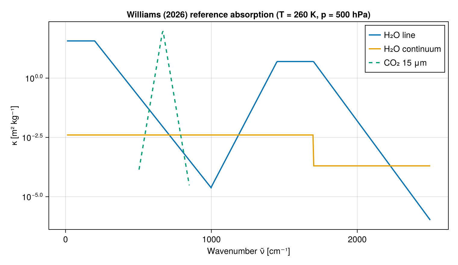
All three curves are evaluated at the paper's reference state (T, p, RH) = (260 K, 500 hPa, 100 %). At runtime williams_optical_depth_increment applies pressure broadening (κ ∝ p / p_ref), continuum temperature scaling (exp(σ_cont (T_ref − T)), Mlawer et al. 1997), and the two-stream diffusivity factor D = 1.5 (Armstrong 1968).
2 × CO₂ clear-sky forcing
A standard clear-sky CO₂-doubling benchmark. The column is a lapse-rate atmosphere from 220 K at the top to 295 K at the surface with constant specific humidity q = 5 g kg⁻¹ and surface pressure 1000 hPa.
using NumericalRadiation
using CairoMakie

Nz = 32
σᵢ = collect(range(0, 1, length=Nz + 1))   # interface sigma coordinate
grid = ColumnGrid(σᵢ)

FT = Float64
surface   = SurfaceState(FT; sea_surface_temperature=295, land_surface_temperature=285, land_fraction=0.3)
constants = PhysicalConstants(FT)
longwave  = AnalyticBandLongwave(FT)

# Sweep CO₂
carbon_dioxide_ppm = [50, 100, 200, 280, 400, 560, 800, 1120]
OLR = FT[]
for CO₂ in carbon_dioxide_ppm
    profile = AtmosphereProfile(
        temperature      = collect(range(220, 295, length=Nz)),
        humidity         = fill(0.005, Nz),
        geopotential     = zeros(Nz),
        surface_pressure = 100_000,
        CO₂              = CO₂,
    )
    Ṫ = zeros(Nz)
    diagnostics = LongwaveDiagnostics(FT)
    solve_longwave!(Ṫ, diagnostics, longwave, profile, grid, surface, constants)
    push!(OLR, diagnostics.outgoing_longwave)
end

fig = Figure(size=(820, 360))
ax1 = Axis(fig[1, 1];
           xlabel = "CO₂ [ppmv]",
           ylabel = "ℐꜛˡʷ at TOA [W m⁻²]",
           xscale = log10,
           title  = "Clear-sky outgoing longwave vs CO₂")
lines!(ax1, carbon_dioxide_ppm, OLR;   color=:black, linestyle=:dash)
scatter!(ax1, carbon_dioxide_ppm, OLR; markersize=10, color=:black)

ax2 = Axis(fig[1, 2];
           xlabel = "CO₂ [ppmv]",
           ylabel = "ℐꜛˡʷ(280) − ℐꜛˡʷ(CO₂) [W m⁻²]",
           xscale = log10,
           title  = "Clear-sky CO₂ radiative forcing")
lines!(ax2, carbon_dioxide_ppm, OLR[4] .- OLR; color=:crimson, linewidth=2)
scatter!(ax2, carbon_dioxide_ppm, OLR[4] .- OLR; markersize=10, color=:crimson)
vlines!(ax2, 560; color=:gray70, linestyle=:dot)
hlines!(ax2, 0;   color=:gray70)

ΔOLR = OLR[4] - OLR[6]
Label(fig[2, 1:2], "2× CO₂ forcing (280 → 560 ppmv) = $(round(ΔOLR, digits = 2)) W m⁻²";
      tellwidth = false, fontsize = 12)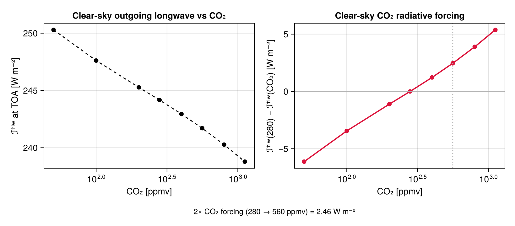
The forcing of OLR(280) − OLR(560) is in the physically plausible range for clear-sky 2×CO₂ (2–5 W m⁻², cf. IPCC AR6 WG1 Ch. 7).