Shortwave: SPEEDY one-band scheme
The OneBandShortwave solver composes three sub-schemes — a diagnostic cloud model, a layer transmissivity, and a radiative-transfer solver — into a single call. It reproduces Fortran SPEEDY (Kucharski, Molteni & Bracco, 2006, Appendix B) with the same parameter defaults.
Transmissivity sensitivity to zenith angle
using NumericalRadiation
using CairoMakie

Nz = 32
σᵢ = collect(range(0, 1, length=Nz + 1))   # interface sigma coordinate
grid = ColumnGrid(σᵢ)

profile = AtmosphereProfile(
    temperature      = collect(range(220, 295, length=Nz)),
    humidity         = fill(0.005, Nz),
    geopotential     = zeros(Nz),
    surface_pressure = 100_000,
)
FT = Float64
constants = PhysicalConstants(FT)
thermo    = ThermodynamicConstants(FT)
scheme    = NumericalRadiation.OneBandShortwave(FT)

zenith_cosines = [0.2, 0.4, 0.6, 0.8, 1]
fig = Figure(size=(780, 420))
ax  = Axis(fig[1, 1];
           xlabel = "SW heating rate [K day⁻¹]",
           ylabel = "σ (nondimensional pressure)",
           yreversed = true,
           title  = "Shortwave heating rate vs zenith angle")

for μ₀ in zenith_cosines
    surface = SurfaceState(FT; sea_surface_temperature = 295,
                           land_surface_temperature = NaN,
                           land_fraction = 0,
                           ocean_albedo = 0.07,
                           land_albedo  = 0.07,
                           cos_zenith   = μ₀)
    Ṫ = zeros(Nz)
    diagnostics = ShortwaveDiagnostics(FT, Nz)
    transmissivity = similar(profile.temperature)
    solve_shortwave!(Ṫ, diagnostics, scheme, profile, grid, surface,
                     constants, thermo; transmissivity_scratch = transmissivity)
    lines!(ax, Ṫ .* 86_400, grid.σ_full; label="μ₀ = $μ₀", linewidth=2)
end
Legend(fig[2, 1], ax; orientation=:horizontal, framevisible=false)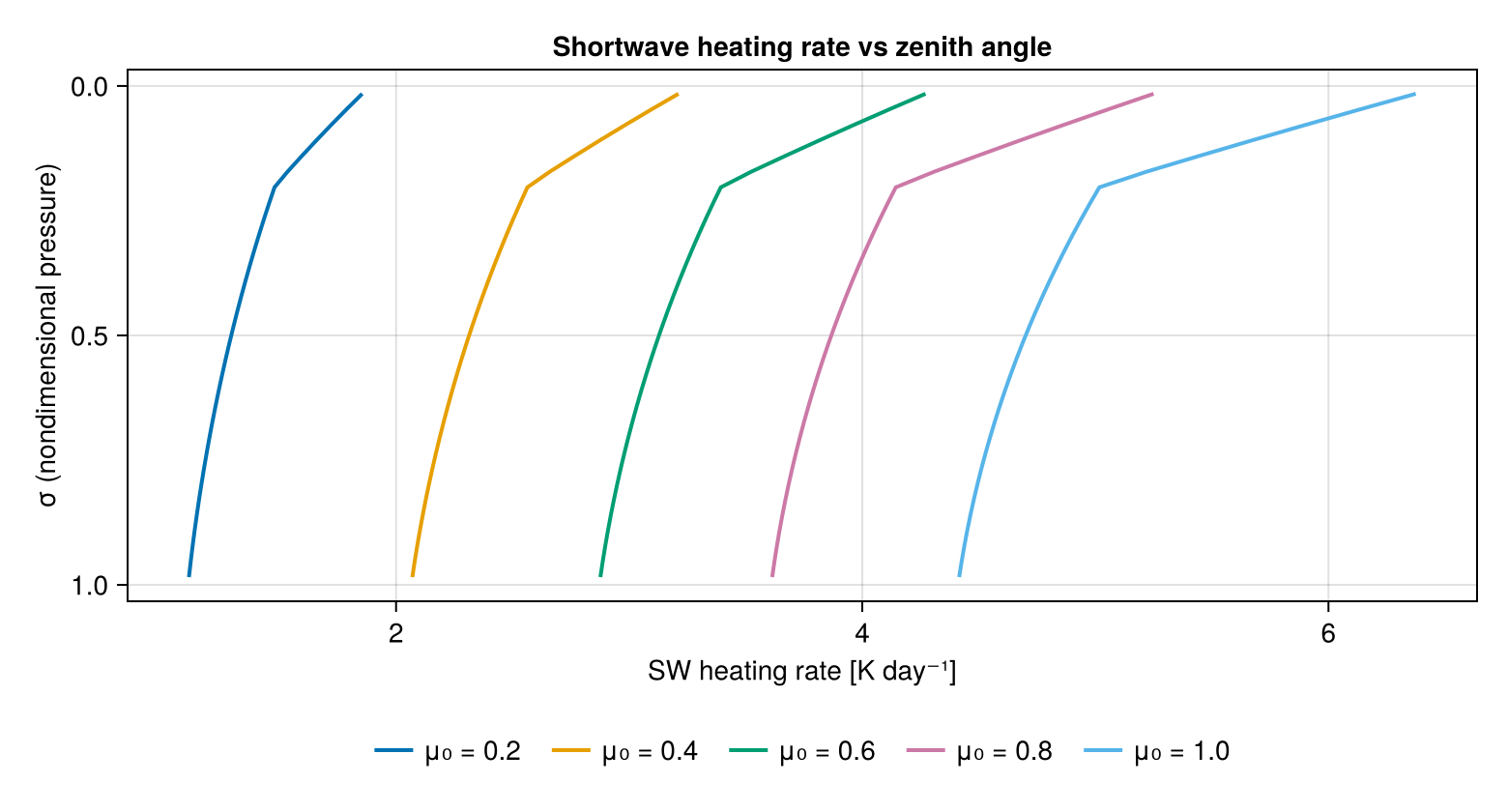
Near the TOA the heating is dominated by ozone; near the surface by water vapour. At grazing angles (μ₀ → 0) the optical path is long and heating is concentrated aloft, matching the SPEEDY zenith-correction factor (1 + a_zen (1 − μ₀)^n_zen) in BackgroundShortwaveTransmissivity.
Cloud-albedo sensitivity
Repeating the same column but sweeping the cloud cover through the diagnostic scheme's precipitation term shows the surface-insolation response.
using NumericalRadiation
using CairoMakie

Nz = 16
σᵢ = collect(range(0, 1, length=Nz + 1))
grid = ColumnGrid(σᵢ)
base_profile = AtmosphereProfile(
    temperature      = collect(range(220, 295, length=Nz)),
    humidity         = fill(0.008, Nz),
    geopotential     = zeros(Nz),
    surface_pressure = 100_000,
)
FT = Float64
surface = SurfaceState(FT; sea_surface_temperature = 295,
                       land_surface_temperature = NaN,
                       land_fraction = 0,
                       ocean_albedo = 0.07,
                       land_albedo  = 0.07,
                       cos_zenith   = 0.6)
constants = PhysicalConstants(FT)
thermo    = ThermodynamicConstants(FT)
scheme    = NumericalRadiation.OneBandShortwave(FT)

rain_rates = [0, 1e-7, 1e-6, 5e-6, 1e-5, 5e-5, 1e-4]   # m/s
surface_down = FT[]
toa_up       = FT[]
cloud_covers = FT[]
for rain_rate in rain_rates
    profile = AtmosphereProfile(temperature = base_profile.temperature,
                                humidity = base_profile.humidity,
                                geopotential = base_profile.geopotential,
                                surface_pressure = base_profile.surface_pressure,
                                rain_rate = rain_rate)
    Ṫ = zeros(Nz)
    diagnostics = ShortwaveDiagnostics(FT, Nz)
    transmissivity = similar(profile.temperature)
    solve_shortwave!(Ṫ, diagnostics, scheme, profile, grid, surface,
                     constants, thermo; transmissivity_scratch = transmissivity)
    push!(surface_down, diagnostics.surface_shortwave_down)
    push!(toa_up, diagnostics.outgoing_shortwave)
    push!(cloud_covers, diagnostics.cloud_cover)
end

fig = Figure(size=(780, 360))
ax  = Axis(fig[1, 1];
           xlabel = "Diagnosed cloud cover",
           ylabel = "Flux [W m⁻²]",
           title  = "Cloud-cover response of SW fluxes")
scatter!(ax, cloud_covers, surface_down; label="ℐꜜˢʷ at surface", markersize=10)
scatter!(ax, cloud_covers, toa_up;       label="ℐꜛˢʷ at TOA",      markersize=10)
axislegend(ax; position=:rc, framevisible=false)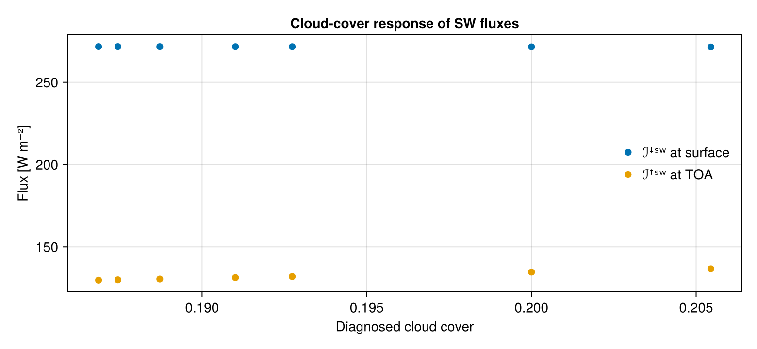
As cloud cover grows, more solar flux is reflected back to space (TOA up rises) and less reaches the surface.