Manabe radiative-convective equilibrium with ecCKD

What surface temperature does an atmospheric column choose, and how much does it warm when CO₂ doubles? Manabe and Wetherald answered those questions in 1967 (J. Atmos. Sci., doi: 10.1175/1520-0469(1967)024<0241:TEOTAW>2.0.CO;2). This page runs a Manabe-style version of that calculation: radiation heats and cools each level, convection instantly clamps the column onto a critical lapse-rate profile anchored at the surface, the surface temperature is solved from top-of-atmosphere energy balance, and — their famous choice — relative humidity stays fixed, so water vapor rises and falls with temperature. The formulation follows the RRTMGP.jl Manabe tutorial: level temperatures are prognostic, convective adjustment is a one-line clamp at a fixed trial surface temperature, and the surface temperature is solved externally from top-of-atmosphere balance. RRTMGP is a source reference only — nothing here imports or calls it.

Configuration

The experiment's headline parameters and physical constants:

using NumericalRadiation
using NCDatasets   # activates the NetCDF loader for the ecCKD file
using Printf

Γ  = 6.5e-3                  # critical lapse rate, K m⁻¹ (Manabe-Wetherald)
μ₀ = cosd(47.9)              # cosine of the solar zenith angle
S₀ = 509                     # solar constant, W m⁻² (Manabe-Wetherald daily mean)
ℐꜜ_toa = S₀ * μ₀             # horizontal TOA shortwave flux, W m⁻²
α  = 0.3                     # surface albedo

surface_relative_humidity = 0.77   # Manabe-Wetherald humidity profile parameter
water_vapor_floor = 4.8e-6         # stratospheric χH₂O floor, mole fraction

χCH₄ = 1.9e-6                # present-day global means for the
χN₂O = 3.4e-7                # well-mixed trace gases

Nz = 60                      # physical layers, uniform in altitude
zₜ = 60e3                    # m; one isothermal lookup-boundary layer above
pˢ = 101_325                 # Pa

constants = PhysicalConstants()      # Earth defaults; every constant below is one of its fields
g  = constants.gravity               # gravitational acceleration, m s⁻²
cᵖ = constants.heat_capacity         # isobaric heat capacity, J kg⁻¹ K⁻¹
σ  = constants.stefan_boltzmann      # Stefan-Boltzmann constant, W m⁻² K⁻⁴
Rᵈ = constants.dry_air_gas_constant  # dry-air gas constant, J kg⁻¹ K⁻¹
mᵈ = constants.dry_air_molar_mass    # dry-air molar mass, kg mol⁻¹
mᵛ = constants.water_molar_mass      # water molar mass, kg mol⁻¹
freezing_temperature = ThermodynamicConstants().freezing_temperature   # K
day = 86_400         # s

The atmospheric profile and grid

The initial state is an analytic midlatitude-summer standard atmosphere, transcribed locally from RRTMGP.jl's standard_atmosphere source (AFGL-style two-segment temperature, exact hydrostatic pressure, and log-pressure-Gaussian ozone). Transcribed, not imported.

T₀             = 294     # K, midlatitude-summer surface temperature
z_tropopause   = 13e3    # m, idealized tropopause height
Γ_stratosphere = 2e-3    # K m⁻¹, idealized stratospheric warming rate

standard_temperature(z) = z <= z_tropopause ? T₀ - Γ * z : (T₀ - Γ * z_tropopause) + Γ_stratosphere * (z - z_tropopause)

function standard_pressure(z)
    T_tropopause = T₀ - Γ * z_tropopause
    z <= z_tropopause && return pˢ * (standard_temperature(z) / T₀)^(g / (Rᵈ * Γ))
    p_tropopause = pˢ * (T_tropopause / T₀)^(g / (Rᵈ * Γ))
    return p_tropopause * (standard_temperature(z) / T_tropopause)^(-g / (Rᵈ * Γ_stratosphere))
end

standard_ozone(p) = 3e-8 + 7.5e-6 * exp(-(log(p / 1_200))^2 / (2 * 1.2^2))

Levels are uniform in altitude from the surface to zₜ, stored TOA-first (our column convention, pressure increasing downward). One separate isothermal lookup-boundary layer spans from the gas-optics table's minimum pressure down to the top physical level; it is excluded from all prognostic, adjustment, and convergence arrays — its temperature and gas state are copied from the top physical level before every radiation call and its heating is discarded. Extension-column arrays carry the suffix _extended; index 1 is the extension layer and physical layer j sits at j + 1.

gas_optics = read_reference_ecckd_gas_optics("32x32"; names=(:composite, :h2o, :o3, :co2, :ch4, :n2o))

zᵢ = collect(range(0, zₜ; length=Nz + 1))
z = 0.5 .* (zᵢ[1:Nz] .+ zᵢ[2:Nz+1])
pᵢ = reverse(standard_pressure.(zᵢ))     # TOA-first, increasing downward
p = reverse(standard_pressure.(z))       # standard_pressure at altitude midpoints

table_minimum_pressure = first(gas_optics.pressure_grid)
table_minimum_pressure < pᵢ[1] || error("lookup-table minimum pressure does not lie above the physical top")

Nz_extended = Nz + 1                                           # extension layer + physical layers
p_extended = vcat(0.5 * (table_minimum_pressure + pᵢ[1]), p)   # arithmetic midpoint
pᵢ_extended = vcat(table_minimum_pressure, pᵢ)                 # for the extension only
χO₃ = standard_ozone.(p)
χO₃_extended = vcat(χO₃[1], χO₃)                               # extension copies the top layer

The humidity closure

Fixed relative humidity on layer temperatures — Manabe and Wetherald's profile shape, Magnus saturation vapor pressure, and a stratospheric floor — applied to the full radiation column including the extension layer:

saturation_vapor_pressure(T) = 610.94 * exp(17.625 * (T - freezing_temperature) / (T - 30.11))

function fixed_relative_humidity!(χH₂O_extended, T_extended)
    for k in eachindex(χH₂O_extended)
        relative_humidity = max(surface_relative_humidity * (p_extended[k] / pˢ - 0.02) / 0.98, 0)
        pᵛ⁺ = saturation_vapor_pressure(T_extended[k])
        χH₂O_extended[k] = max(relative_humidity * pᵛ⁺ / max(p_extended[k] - relative_humidity * pᵛ⁺, 1),
                               water_vapor_floor)
    end
    return χH₂O_extended
end

Radiation work arrays

The staged runtime operates on caller-owned arrays: per-g-point optical properties for each band, and broadband fluxes on the interfaces.

function radiation_work_arrays(gas_optics, Nz)
    Ngˡʷ = length(gas_optics.longwave_weights)
    Ngˢʷ = length(gas_optics.shortwave_weights)
    longwave = LongwaveOptics(zeros(Ngˡʷ, Nz),
                              zeros(Ngˡʷ, Nz);
                              source_top = zeros(Ngˡʷ, Nz),
                              source_bottom = zeros(Ngˡʷ, Nz),
                              weights = zeros(Ngˡʷ))
    shortwave = ShortwaveOptics(zeros(Ngˢʷ, Nz);
                                rayleigh_optical_depth = zeros(Ngˢʷ, Nz),
                                scattering_asymmetry = zeros(Ngˢʷ, Nz),
                                weights = zeros(Ngˢʷ))
    fluxes = RadiativeFluxes(longwave_up = zeros(Nz + 1),
                             longwave_down = zeros(Nz + 1),
                             shortwave_up = zeros(Nz + 1),
                             shortwave_down = zeros(Nz + 1))
    return longwave, shortwave, fluxes
end

The radiative-convective march

equilibrate! marches the column at a fixed trial surface temperature, in the RRTMGP tutorial's exact order and stopping rule: clamp levels onto the critical profile $T_c(p) = Tˢ (p/pˢ)^{Γ R^{\mathrm{d}}/g}$; set layer temperatures to adjacent-level means; update humidity and fluxes; stop when one successive adjusted level profile changes by less than tolerance (kelvin); otherwise map layer heating to level tendencies (interior levels take the mean of the adjacent layer rates, the end levels take the edge rate) and march with the tutorial's ±2 K increment clamp, up to max_steps steps.

function equilibrate!(Tᵢ, Tˢ; χCO₂, ozone = χO₃_extended, fixed_water_vapor = nothing,
                      Δt = 8 * 3_600, max_steps = 20_000, tolerance = 1e-4)
    T_extended = zeros(Nz_extended)
    Tᵢ_extended = zeros(Nz_extended + 1)
    χH₂O_extended = zeros(Nz_extended)
    nᵈ = zeros(Nz_extended)
    gases = (composite = zeros(Nz_extended), h2o = zeros(Nz_extended), o3 = zeros(Nz_extended),
             co2 = zeros(Nz_extended), ch4 = zeros(Nz_extended), n2o = zeros(Nz_extended))
    atmosphere = ColumnAtmosphere(; pressure_layers = p_extended,
                                    pressure_interfaces = pᵢ_extended,
                                    temperature_layers = T_extended,
                                    temperature_interfaces = Tᵢ_extended,
                                    gases, surface = nothing,
                                    geometry = (cos_zenith=μ₀,),
                                    constants)
    longwave, shortwave, fluxes = radiation_work_arrays(gas_optics, Nz_extended)
    shortwave_boundary = ShortwaveBoundaryConditions(toa_shortwave_down=ℐꜜ_toa, surface_albedo=α)
    surface_emission = surface_longwave_emission(gas_optics, Tˢ)
    longwave_boundary = LongwaveBoundaryConditions(surface_longwave_up=surface_emission)
    Q = zeros(Nz_extended)
    Ṫᵢ = zeros(Nz + 1)
    previous = zeros(Nz + 1)

    solve_radiation!() = begin
        # extension layer: isothermal with, and gas state tied to, the top level
        T_extended[1] = Tᵢ[1]
        @views @. T_extended[2:Nz_extended] = (Tᵢ[1:Nz] + Tᵢ[2:Nz+1]) / 2
        Tᵢ_extended[1] = Tᵢ[1]
        @views Tᵢ_extended[2:Nz_extended+1] .= Tᵢ
        if isnothing(fixed_water_vapor)
            fixed_relative_humidity!(χH₂O_extended, T_extended)
        else
            χH₂O_extended .= fixed_water_vapor
        end
        χH₂O_extended[1] = χH₂O_extended[2]      # extension copies the top physical layer
        for k in 1:Nz_extended
            nᵈ[k] = (pᵢ_extended[k + 1] - pᵢ_extended[k]) / (g * (mᵈ + mᵛ * χH₂O_extended[k]))
            gases.composite[k] = nᵈ[k]
            gases.h2o[k] = χH₂O_extended[k] * nᵈ[k]
            gases.o3[k] = ozone[k] * nᵈ[k]
            gases.co2[k] = χCO₂ * nᵈ[k]
            gases.ch4[k] = χCH₄ * nᵈ[k]
            gases.n2o[k] = χN₂O * nᵈ[k]
        end
        optical_properties!(longwave, shortwave, gas_optics, atmosphere)
        radiative_fluxes!(fluxes, CloudlessLongwave(), longwave, atmosphere, longwave_boundary)
        radiative_fluxes!(fluxes, CloudlessShortwave(), shortwave, atmosphere, shortwave_boundary)
    end

    critical = Tˢ .* (pᵢ ./ pˢ) .^ (Γ * Rᵈ / g)
    fill!(previous, 0)
    final_difference = Inf
    steps = max_steps
    converged = false
    for step in 1:max_steps
        @. Tᵢ = max(Tᵢ, critical)
        solve_radiation!()
        final_difference = maximum(abs, Tᵢ .- previous)
        if final_difference < tolerance
            steps = step
            converged = true
            break
        end
        previous .= Tᵢ
        heating_rates!(Q, fluxes, atmosphere)     # g and cᵖ from atmosphere.constants
        # discard the extension tendency Q[1]; physical layer j is Q[j + 1]
        Ṫᵢ[1] = Q[2]
        Ṫᵢ[Nz+1] = Q[Nz_extended]
        @views @. Ṫᵢ[2:Nz] = (Q[2:Nz_extended-1] + Q[3:Nz_extended]) / 2
        @. Tᵢ += clamp(Δt * Ṫᵢ, -2, 2)
    end
    return (; Tᵢ = copy(Tᵢ), Tˢ, converged, final_difference, steps,
              days = steps * Δt / day,
              χH₂O = copy(χH₂O_extended),
              T_extended = copy(T_extended),
              extension_temperature = T_extended[1],
              olr = fluxes.longwave_up[1],
              asr = fluxes.shortwave_down[1] - fluxes.shortwave_up[1])
end

The energy-balance solve

rce wraps the march in a safeguarded root solve for ASR − OLR = 0. The generic bookkeeping expands the initial guesses (doubling, hard-bounded to [150, 350] K) until the imbalance changes sign, then iterates a secant step with a bisection fallback:

function bracketed_secant(toa_imbalance, guesses; imbalance_tolerance=0.1, max_expansions=8, max_iterations=12)
    lower, upper = min(guesses...), max(guesses...)
    ΔF_lower, state_lower = toa_imbalance(lower)
    ΔF_upper, state_upper = toa_imbalance(upper)
    expansion = 8
    expansions = 0
    while sign(ΔF_lower) == sign(ΔF_upper)
        expansions < max_expansions || error("no sign-changing Tˢ bracket after $max_expansions expansions")
        saturated = lower == 150 && upper == 350
        saturated && error("Tˢ bracket saturated the [150, 350] K domain without a sign change")
        lower = max(lower - expansion, 150)
        upper = min(upper + expansion, 350)
        expansion *= 2
        expansions += 1
        ΔF_lower, state_lower = toa_imbalance(lower)
        ΔF_upper, state_upper = toa_imbalance(upper)
    end
    Tˢ, ΔF, state = abs(ΔF_lower) < abs(ΔF_upper) ? (lower, ΔF_lower, state_lower) : (upper, ΔF_upper, state_upper)
    a, b, ΔF_a, ΔF_b = lower, upper, ΔF_lower, ΔF_upper
    iterations = 0
    step_size = Inf
    while abs(ΔF) > imbalance_tolerance || step_size > 0.01
        iterations < max_iterations || error("surface-temperature solve exceeded $max_iterations iterations")
        candidate = ΔF_b == ΔF_a ? (a + b) / 2 : b - ΔF_b * (b - a) / (ΔF_b - ΔF_a)
        (a < candidate < b) || (candidate = (a + b) / 2)
        ΔF_c, state_c = toa_imbalance(candidate)
        if sign(ΔF_c) == sign(ΔF_a)
            a, ΔF_a = candidate, ΔF_c
        else
            b, ΔF_b = candidate, ΔF_c
        end
        step_size = abs(candidate - Tˢ)
        Tˢ, ΔF, state = candidate, ΔF_c, state_c
        iterations += 1
    end
    return Tˢ, state, iterations, expansions
end

function rce(χCO₂; ozone = χO₃_extended, fixed_water_vapor = nothing,
             Tˢ_guesses = (285, 295), warm_start = nothing,
             imbalance_tolerance = 0.1, max_expansions = 8, max_iterations = 12)
    Tᵢ = isnothing(warm_start) ? standard_temperature.(reverse(zᵢ)) : copy(warm_start)
    toa_imbalance(Tˢ) = begin
        state = equilibrate!(Tᵢ, Tˢ; χCO₂, ozone, fixed_water_vapor)
        state.converged || error("inner equilibration at trial Tˢ = $Tˢ did not converge")
        ΔF = state.asr - state.olr
        isfinite(ΔF) || error("nonfinite TOA residual at trial Tˢ = $Tˢ")
        (ΔF, state)
    end
    Tˢ, state, iterations, expansions = bracketed_secant(toa_imbalance, Tˢ_guesses; imbalance_tolerance,
                                                         max_expansions, max_iterations)
    return (; state..., Tˢ, secant_iterations=iterations, bracket_expansions=expansions)
end

The experiments, and the answer

The main experiment runs 1×, 2×, and 4× CO₂ with the fixed-RH closure, plus the discriminating control: 4× CO₂ with water vapor frozen at the control field. Every equilibration must pass the verification gates at the end of this page, or the page fails to build.

χCO₂ = 420e-6

control      = rce(χCO₂)
doubled      = rce(2χCO₂; warm_start=control.Tᵢ)
quadrupled   = rce(4χCO₂; warm_start=control.Tᵢ)
frozen_vapor = rce(4χCO₂; warm_start=control.Tᵢ, fixed_water_vapor=control.χH₂O)

for (name, state) in (("control, 420 ppm CO₂", control),
                      ("2× CO₂, fixed RH", doubled),
                      ("4× CO₂, fixed RH", quadrupled),
                      ("4× CO₂, frozen water vapor", frozen_vapor))
    @printf("%-28s Tˢ = %7.2f K   ΔTˢ = %+6.2f K\n", name, state.Tˢ, state.Tˢ - control.Tˢ)
end

control, 420 ppm CO₂         Tˢ =  288.09 K   ΔTˢ =  +0.00 K
2× CO₂, fixed RH             Tˢ =  290.72 K   ΔTˢ =  +2.63 K
4× CO₂, fixed RH             Tˢ =  293.85 K   ΔTˢ =  +5.77 K
4× CO₂, frozen water vapor   Tˢ =  291.11 K   ΔTˢ =  +3.02 K

Comparing the two 4× equilibria isolates the fixed-RH water-vapor amplification in this configuration: the same quadrupled CO₂ warms the surface nearly twice as much when the vapor is allowed to rise with temperature as when it is frozen at the control field.

The solver marches level temperatures; the figures show the derived layer-center profiles, where gas optical properties and heating rates are evaluated, as the current RRTMGP tutorial does.

using CairoMakie

pressure_ticks = ([0.3, 1, 3, 10, 30, 100, 300, 1000], ["0.3", "1", "3", "10", "30", "100", "300", "1000"])

function profile_axis(fig; title)
    return Axis(fig[1, 1]; xlabel = "Temperature (K)", ylabel = "Pressure (hPa)",
                yscale = log10, yreversed = true,
                yticks = pressure_ticks, title)
end

fig = Figure(size=(700, 660))
ax = profile_axis(fig; title="RCE response to CO₂")
for (state, label, color, style) in
        ((control, "1× CO₂ (420 ppm), fixed RH", :steelblue4, :solid),
         (doubled, "2× CO₂, fixed RH", :darkorange3, :solid),
         (quadrupled, "4× CO₂, fixed RH", :firebrick, :solid),
         (frozen_vapor, "4× CO₂, frozen water vapor", :firebrick, :dash))
    lines!(ax, state.T_extended[2:Nz_extended], p ./ 100; color, label, linewidth=2, linestyle=style)
    scatter!(ax, [state.Tˢ], [pˢ / 100]; color, markersize=10)
end
Legend(fig[2, 1], ax; orientation=:horizontal, nbanks=2, framevisible=false)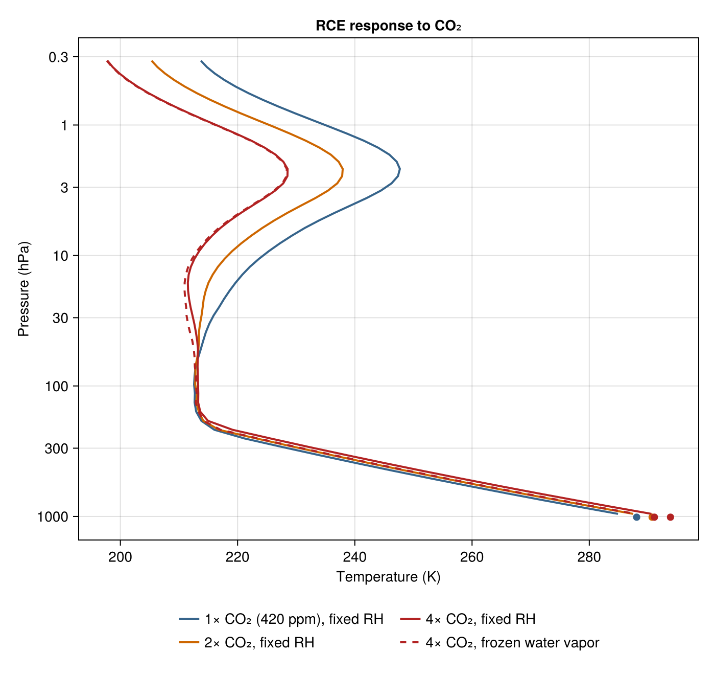

A troposphere on the critical lapse-rate profile anchored at the solved surface temperature (marked at the bottom), a tropopause, and a stratosphere in radiative equilibrium. CO₂ warms the coupled surface-troposphere state while cooling the stratosphere, and the dashed frozen-vapor state shows how much smaller the same 4× forcing leaves the response when vapor cannot rise with temperature.

What each absorber contributes

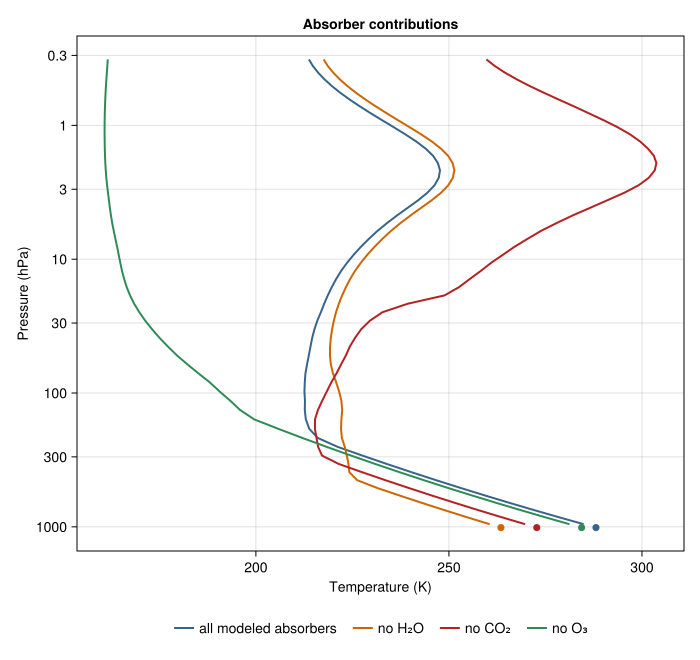
A companion RCE experiment removes one absorber at a time and re-solves the full equilibrium — water vapor frozen to zero, CO₂ removed, or ozone removed, each through the same solver and gates:

without_H₂O = rce(χCO₂; warm_start=control.Tᵢ, fixed_water_vapor=zero(control.χH₂O), Tˢ_guesses=(255, 275))
without_CO₂ = rce(0; warm_start=control.Tᵢ, Tˢ_guesses=(265, 285))
without_O₃  = rce(χCO₂; warm_start=control.Tᵢ, ozone=zero(χO₃_extended), Tˢ_guesses=(275, 292))

for (name, state) in (("without water vapor", without_H₂O), ("without CO₂", without_CO₂), ("without O₃", without_O₃))
    @printf("%-28s Tˢ = %7.2f K   ΔTˢ = %+6.2f K\n", name, state.Tˢ, state.Tˢ - control.Tˢ)
end

fig = Figure(size=(700, 660))
ax = profile_axis(fig; title="Absorber contributions")
for (state, label, color) in
        ((control, "all modeled absorbers", :steelblue4),
         (without_H₂O, "no H₂O", :darkorange3),
         (without_CO₂, "no CO₂", :firebrick),
         (without_O₃, "no O₃", :seagreen))
    lines!(ax, state.T_extended[2:Nz_extended], p ./ 100; color, label, linewidth=2)
    scatter!(ax, [state.Tˢ], [pˢ / 100]; color, markersize=10)
end
Legend(fig[2, 1], ax; orientation=:horizontal, framevisible=false)

without water vapor          Tˢ =  263.47 K   ΔTˢ = -24.62 K
without CO₂                  Tˢ =  272.75 K   ΔTˢ = -15.33 K
without O₃                   Tˢ =  284.37 K   ΔTˢ =  -3.72 K

Verification

Every equilibrium on this page must pass these build-failing gates: inner convergence, top-of-atmosphere closure, layer/level consistency, the isothermal lookup-boundary layer, a tropospheric inversion limit, and surface-emission consistency.

function verify_equilibria(states; imbalance_gate=0.1)
    for (name, state) in states
        state.converged || error("$name: final equilibration not converged")
        abs(state.asr - state.olr) < imbalance_gate || error("$name: TOA imbalance $(state.asr - state.olr) W/m²")
        layer_means = (state.Tᵢ[1:Nz] .+ state.Tᵢ[2:Nz+1]) ./ 2
        isequal(layer_means, state.T_extended[2:Nz_extended]) ||
            error("$name: layer temperatures are not adjacent-level means")
        state.extension_temperature == state.Tᵢ[1] ||
            error("$name: lookup-boundary layer is not isothermal with the top level")
        inversion_limit = minimum(diff(state.Tᵢ)[pᵢ[1:Nz] .> 40_000])
        inversion_limit > -0.05 || error("$name: tropospheric inversion-limit gate: $(inversion_limit) K per level")
    end
    reference_state = states[1][2]
    weighted_emission = sum(gas_optics.longwave_weights .* surface_longwave_emission(gas_optics, reference_state.Tˢ))
    abs(weighted_emission - σ * reference_state.Tˢ^4) < 0.2 || error("weighted surface emission inconsistent with σTˢ⁴")
    return nothing
end

verify_equilibria([("control", control), ("2×", doubled),
                   ("4×", quadrupled), ("4× frozen vapor", frozen_vapor),
                   ("no H₂O", without_H₂O), ("no CO₂", without_CO₂),
                   ("no O₃", without_O₃)])

Three ideas behind the calculation

Radiative equilibrium alone would make each level's temperature settle where its absorption of solar and terrestrial radiation balances its own emission — producing an unstably steep profile in the lower atmosphere. Convective adjustment is the instantaneous limit of the convection that such a profile would trigger: any level colder than the critical profile $T_c(p) = Tˢ (p/pˢ)^{Γ R^{\mathrm{d}}/g}$ anchored at the surface is clamped onto it, so the troposphere rides the critical lapse rate over a radiatively balanced stratosphere while the surface temperature itself is solved from top-of-atmosphere balance. The fixed-RH humidity closure is Manabe and Wetherald's third ingredient: holding relative humidity fixed means a warmer column holds more vapor — itself a greenhouse gas — so any CO₂-driven warming is amplified, which the frozen-vapor control isolates by turning exactly that closure off.

This page was generated using Literate.jl.