Single-column analytical radiation

This page drives the analytical longwave and shortwave solvers together on a single column and plots their heating-rate profiles. It serves as a template for integrating NumericalRadiation into a single-column model or for debugging a new band parameterization.

Lapse-rate column, daytime + doubled CO₂

using NumericalRadiation
using CairoMakie

Nz = 32
σᵢ = collect(range(0, 1, length=Nz + 1))   # interface sigma coordinate
grid = ColumnGrid(σᵢ)

base_profile = AtmosphereProfile(
    temperature      = collect(range(220, 295, length=Nz)),
    humidity         = fill(0.008, Nz),
    geopotential     = zeros(Nz),
    surface_pressure = 100_000,
)
FT = Float64
surface = SurfaceState(FT; sea_surface_temperature = 295,
                       land_surface_temperature = NaN,
                       land_fraction = 0,
                       ocean_albedo = 0.07,
                       land_albedo  = 0.07,
                       cos_zenith   = 0.5)
constants = PhysicalConstants(FT)
thermo    = ThermodynamicConstants(FT)

longwave  = AnalyticBandLongwave(FT)
shortwave = NumericalRadiation.OneBandShortwave(FT)

function solve_column(carbon_dioxide_ppmv)
    profile = AtmosphereProfile(
        temperature      = base_profile.temperature,
        humidity         = base_profile.humidity,
        geopotential     = base_profile.geopotential,
        surface_pressure = base_profile.surface_pressure,
        CO₂              = carbon_dioxide_ppmv,
    )
    Ṫˡʷ = zeros(Nz)
    Ṫˢʷ = zeros(Nz)
    longwave_diagnostics  = LongwaveDiagnostics(FT)
    shortwave_diagnostics = ShortwaveDiagnostics(FT, Nz)
    transmissivity = similar(profile.temperature)

    solve_longwave!(Ṫˡʷ, longwave_diagnostics, longwave, profile, grid, surface, constants)
    solve_shortwave!(Ṫˢʷ, shortwave_diagnostics, shortwave, profile, grid,
                     surface, constants, thermo;
                     transmissivity_scratch = transmissivity)
    return (; Ṫˡʷ, Ṫˢʷ, longwave_diagnostics, shortwave_diagnostics)
end

baseline = solve_column(280)
doubled  = solve_column(560)

fig = Figure(size=(920, 460))
ax_longwave = Axis(fig[1, 1]; xlabel="LW heating rate [K day⁻¹]", ylabel="σ", yreversed=true, title="Longwave")
ax_shortwave = Axis(fig[1, 2]; xlabel = "SW heating rate [K day⁻¹]",
                    ylabel = "σ", yreversed = true, title = "Shortwave")
ax_net = Axis(fig[1, 3]; xlabel="Net heating rate [K day⁻¹]", ylabel="σ", yreversed=true, title="Net (LW + SW)")

for (result, label, color) in ((baseline, "280 ppmv", :dodgerblue), (doubled, "560 ppmv", :crimson))
    lines!(ax_longwave, result.Ṫˡʷ .* 86_400, grid.σ_full; label, color, linewidth=2)
    lines!(ax_shortwave, result.Ṫˢʷ .* 86_400, grid.σ_full; label, color, linewidth=2)
    lines!(ax_net, (result.Ṫˡʷ .+ result.Ṫˢʷ) .* 86_400, grid.σ_full; label, color, linewidth=2)
end
Legend(fig[2, 1:3], ax_longwave; orientation=:horizontal, framevisible=false)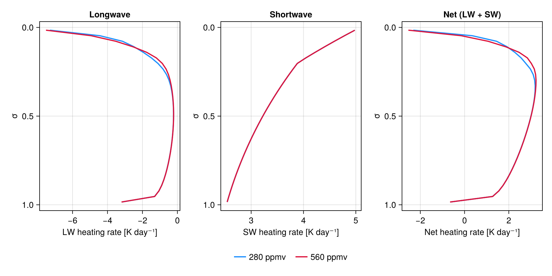

The longwave panel shows the characteristic cooling-to-space signature with stronger cooling where water vapour is most abundant. The shortwave panel shows the ozone bump near the top of the model and the warming contribution from water-vapour near-IR absorption in the lower troposphere. Doubling CO₂ reduces outgoing longwave (more negative LW heating is damped) and leaves the shortwave essentially unchanged.

TOA energy budget

Print the fluxes for each experiment:

for (label, result) in (("280 ppmv", baseline), ("560 ppmv", doubled))
    @info(label,
          olr = result.longwave_diagnostics.outgoing_longwave,
          surface_lw_down = result.longwave_diagnostics.surface_longwave_down,
          toa_sw_up = result.shortwave_diagnostics.outgoing_shortwave,
          surface_sw_down = result.shortwave_diagnostics.surface_shortwave_down)
end

┌ Info: 280 ppmv
│   olr = 217.65902626281527
│   surface_lw_down = 348.33360995188474
│   toa_sw_up = 82.02504015011455
└   surface_sw_down = 213.51439326531658
┌ Info: 560 ppmv
│   olr = 215.769400645381
│   surface_lw_down = 350.11440371247846
│   toa_sw_up = 82.02504015011455
└   surface_sw_down = 213.51439326531658